Factor division Let X and Y be disjoint set of variables Consider - - PDF document

1

• Clique Trees 3

Let’s get BP right

Undirected Graphical Models

Here the couples get to swing!

Graphical Models – 10708 Carlos Guestrin Carnegie Mellon University October 25th, 2006

Readings: K&F: 9.1, 9.2, 9.3, 9.4 K&F: 5.1, 5.2, 5.3, 5.4, 5.5, 5.6

10-708 – Carlos Guestrin 2006

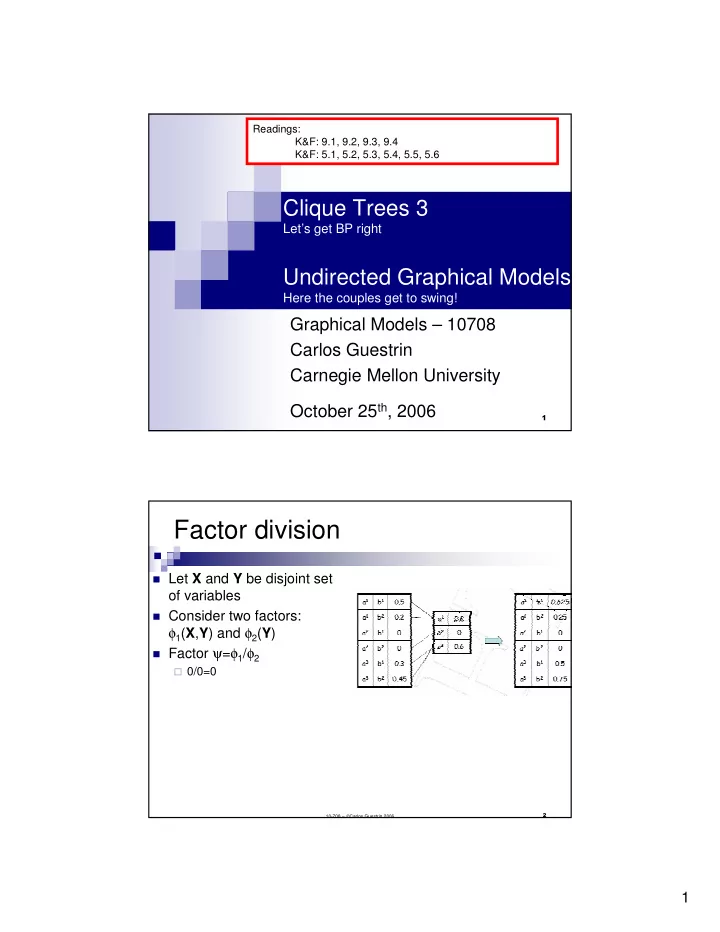
• Factor division

Let X and Y be disjoint set

• f variables

Consider two factors:

φ1(X,Y) and φ2(Y)

Factor ψ=φ1/φ2

0/0=0

2

10-708 – Carlos Guestrin 2006

• Introducing message passing with division

Variable elimination (message passing

with multiplication)

message: belief:

Message passing with division:

message: belief update:

C2: SE C4: GJS C1: CD C3: GDS

10-708 – Carlos Guestrin 2006

• Separator potentials µij
• ne per edge (same both directions)

holds “last message” initialized to 1

Message ij

what does i think the separator potential

should be?

σij

update belief for j:

pushing j to what i thinks about separator

replace separator potential:

C2: SE C4: GJS C1: CD C3: GDS

Lauritzen-Spiegelhalter Algorithm (a.k.a. belief propagation)

3

10-708 – Carlos Guestrin 2006

• Clique tree invariant

Clique tree potential:

Product of clique potentials divided by separators potentials

Clique tree invariant:

P(X) = πΤ (X)

10-708 – Carlos Guestrin 2006

• Belief propagation and clique tree

invariant

Theorem: Invariant is maintained by BP algorithm! BP reparameterizes clique potentials and

separator potentials

At convergence, potentials and messages are marginal

distributions

4

10-708 – Carlos Guestrin 2006

• Subtree correctness

Informed message from i to j, if all messages into i

(other than from j) are informed

Recursive definition (leaves always send informed

messages)

Informed subtree:

All incoming messages informed

Theorem:

Potential of connected informed subtree T’ is marginal over

scope[T’]

Corollary:

At convergence, clique tree is calibrated

πi = P(scope[πi]) µij = P(scope[µij])

10-708 – Carlos Guestrin 2006

• Clique trees versus VE

Clique tree advantages

Multi-query settings Incremental updates Pre-computation makes complexity explicit

Clique tree disadvantages

Space requirements – no factors are “deleted” Slower for single query Local structure in factors may be lost when they are

multiplied together into initial clique potential

5

10-708 – Carlos Guestrin 2006

• Clique tree summary

Solve marginal queries for all variables in only twice the

cost of query for one variable

Cliques correspond to maximal cliques in induced graph Two message passing approaches

VE (the one that multiplies messages) BP (the one that divides by old message)

Clique tree invariant

Clique tree potential is always the same We are only reparameterizing clique potentials

Constructing clique tree for a BN

from elimination order from triangulated (chordal) graph

Running time (only) exponential in size of largest clique

Solve exactly problems with thousands (or millions, or more) of

variables, and cliques with tens of nodes (or less)

10-708 – Carlos Guestrin 2006

• Announcements

Recitation tomorrow, don’t miss it!!!

Khalid on Undirected Models

6

10-708 – Carlos Guestrin 2006

• Swinging Couples revisited

This is no perfect map in BNs But, an undirected model will be a perfect map

10-708 – Carlos Guestrin 2006

• Potentials (or Factors) in Swinging

Couples

7

10-708 – Carlos Guestrin 2006

• Computing probabilities in Markov

networks v. BNs

In a BN, can compute prob. of an

instantiation by multiplying CPTs

In an Markov networks, can only

compute ratio of probabilities directly

10-708 – Carlos Guestrin 2006

• Normalization for computing

probabilities

• To compute actual probabilities, must compute

normalization constant (also called partition function)

• Computing partition function is hard! Must sum over

all possible assignments

8

10-708 – Carlos Guestrin 2006

• Factorization in Markov networks
• Given an undirected graph H over variables

X={X1,...,Xn}

• A distribution P factorizes over H if

subsets of variables D1X,…, DmX, such that the Di

are fully connected in H

non-negative potentials (or factors) π1(D1),…, πm(Dm)

• also known as clique potentials

such that

• Also called Markov random field H, or Gibbs

distribution over H

10-708 – Carlos Guestrin 2006

• Global Markov assumption in

Markov networks

A path X1 – … – Xk is active when set of

variables Z are observed if none of Xi {X1,…,Xk} are observed (are part of Z)

Variables X are separated from Y given Z in

graph H, sepH(X;Y|Z), if there is no active path between any XX and any YY given Z

The global Markov assumption for a Markov

network H is

9

10-708 – Carlos Guestrin 2006

• The BN Representation Theorem

Joint probability distribution:

Obtain

If conditional independencies in BN are subset of conditional independencies in P

Important because: Independencies are sufficient to obtain BN structure G

If joint probability distribution:

Obtain

Then conditional independencies in BN are subset of conditional independencies in P

Important because: Read independencies of P from BN structure G

10-708 – Carlos Guestrin 2006

• Markov networks representation Theorem 1

If you can write distribution as a normalized product of

factors Can read independencies from graph Then

H is an I-map for P If joint probability distribution P:

10

10-708 – Carlos Guestrin 2006

• What about the other direction for Markov

networks ?

Counter-example: X1,…,X4 are binary, and only eight assignments

have positive probability:

For example, X1⊥X3|X2,X4: But distribution doesn’t factorize!!!

If H is an I-map for P

Then

joint probability distribution P:

10-708 – Carlos Guestrin 2006

• Markov networks representation Theorem 2

(Hammersley-Clifford Theorem)

Positive distribution and independencies P factorizes

• ver graph

If H is an I-map for P and P is a positive distribution

Then

joint probability distribution P:

11

10-708 – Carlos Guestrin 2006

• Representation Theorem for

Markov Networks

If H is an I-map for P and P is a positive distribution

Then

joint probability distribution P:

Then

H is an I-map for P If joint probability distribution P:

10-708 – Carlos Guestrin 2006

• Completeness of separation in

Markov networks

Theorem: Completeness of separation

For “almost all” distributions that P factorize over Markov

network H, we have that I(H) = I(P)

“almost all” distributions: except for a set of measure zero of

parameterizations of the Potentials (assuming no finite set of parameterizations has positive measure)

Analogous to BNs

12

10-708 – Carlos Guestrin 2006

• What are the “local” independence

assumptions for a Markov network?

In a BN G:

local Markov assumption: variable independent of

non-descendants given parents

d-separation defines global independence Soundness: For all distributions:

In a Markov net H:

Separation defines global independencies What are the notions of local independencies?

10-708 – Carlos Guestrin 2006

• Local independence assumptions

for a Markov network

Separation defines global independencies Pairwise Markov Independence:

Pairs of non-adjacent variables are independent given all others

Markov Blanket:

Variable independent of rest given its neighbors

T1 T3 T4 T5 T6 T2 T7 T8 T9

13

10-708 – Carlos Guestrin 2006

• Equivalence of independencies in

Markov networks

Soundness Theorem: For all positive distributions P,

the following three statements are equivalent:

P entails the global Markov assumptions P entails the pairwise Markov assumptions P entails the local Markov assumptions (Markov blanket)

10-708 – Carlos Guestrin 2006

• Minimal I-maps and Markov

Networks

A fully connected graph is an I-map Remember minimal I-maps?

A “simplest” I-map Deleting an edge makes it no longer an I-map

In a BN, there is no unique minimal I-map Theorem: In a Markov network, minimal I-map is unique!! Many ways to find minimal I-map, e.g.,

Take pairwise Markov assumption: If P doesn’t entail it, add edge:

14

10-708 – Carlos Guestrin 2006

• How about a perfect map?

Remember perfect maps?

independencies in the graph are exactly the same as those in P

For BNs, doesn’t always exist

counter example: Swinging Couples

How about for Markov networks?

10-708 – Carlos Guestrin 2006

• Unifying properties of BNs and MNs

BNs:

give you: V-structures, CPTs are conditional probabilities, can

directly compute probability of full instantiation

but: require acyclicity, and thus no perfect map for swinging

couples

MNs:

give you: cycles, and perfect maps for swinging couples but: don’t have V-structures, cannot interpret potentials as

probabilities, requires partition function

Remember PDAGS???

skeleton + immoralities provides a (somewhat) unified representation see book for details

15

10-708 – Carlos Guestrin 2006

• What you need to know so far

about Markov networks

Markov network representation:

undirected graph potentials over cliques (or sub-cliques) normalize to obtain probabilities need partition function

Representation Theorem for Markov networks

if P factorizes, then it’s an I-map if P is an I-map, only factorizes for positive distributions

Independence in Markov nets:

active paths and separation pairwise Markov and Markov blanket assumptions equivalence for positive distributions

Minimal I-maps in MNs are unique Perfect maps don’t always exist

10-708 – Carlos Guestrin 2006

• Some common Markov networks

and generalizations

Pairwise Markov networks A very simple application in computer vision Logarithmic representation Log-linear models Factor graphs

16

10-708 – Carlos Guestrin 2006

• Pairwise Markov Networks

All factors are over single variables or pairs of

variables:

Node potentials Edge potentials

Factorization: Note that there may be bigger cliques in the

graph, but only consider pairwise potentials

T1 T3 T4 T5 T6 T2 T7 T8 T9

10-708 – Carlos Guestrin 2006

• A very simple vision application

Image segmentation: separate foreground from

background

Graph structure:

pairwise Markov net grid with one node per pixel

Node potential:

“background color” v. “foreground color”

Edge potential:

neighbors like to be of the same class

17

10-708 – Carlos Guestrin 2006

• Logarithmic representation

Standard model: Log representation of potential (assuming positive potential):

also called the energy function

Log representation of Markov net:

10-708 – Carlos Guestrin 2006

• Log-linear Markov network

(most common representation)

Feature is some function φ[D] for some subset of variables D

e.g., indicator function

Log-linear model over a Markov network H:

a set of features φ1[D1],…, φk[Dk]

each Di is a subset of a clique in H two φ’s can be over the same variables

a set of weights w1,…,wk

usually learned from data

18

10-708 – Carlos Guestrin 2006

• Structure in cliques

Possible potentials for this graph:

A B C

10-708 – Carlos Guestrin 2006

• Factor graphs

Very useful for approximate inference

Make factor dependency explicit

Bipartite graph:

variable nodes (ovals) for X1,…,Xn factor nodes (squares) for φ1,…,φm edge Xi – φj if Xi Scope[φj]

A B C

19

10-708 – Carlos Guestrin 2006

• Summary of types of Markov nets

Pairwise Markov networks

very common potentials over nodes and edges

Log-linear models

log representation of potentials linear coefficients learned from data most common for learning MNs

Factor graphs

explicit representation of factors

you know exactly what factors you have

very useful for approximate inference