f g u ,v = u f x , y g u x ,v y dx dy v Or, in - - PDF document

Programming Example: Filter Operations Hannes Hofmann

Programming Example: Filter Operations

MB-JASS 2006, 19 – 29 March 2006

Convolution

The convolution expresses the amount of overlap of one function g as it is shifted over another function f . Basically it is a product of f and g :  f ∗gu ,v=∫

u ∫ v

f x , yg u− x ,v−ydx dy Or, in the discrete case: cx , y=∑

i=0 n

∑

j=0 n

f x1−i , y1− jk i , j where n denotes the dimension of the filter kernel. Typical filter kernels have a size of 3x3 or 5x5, but larger ones are of cause also possible. If both, signal and filter kernel, are Fourier transformed the convolution becomes a (complex)

• multiplication. In case of large kernels (e.g. Shepp-Logan which is line-long) this "trick" really can

save time. FFT the kernel for each signal FFT the signal multiply signal and kernel element-wise IFFT the signal For the rest of this talk I will use discrete 3x3 convolution in spatial domain unless mentioned.

Example: Convolution

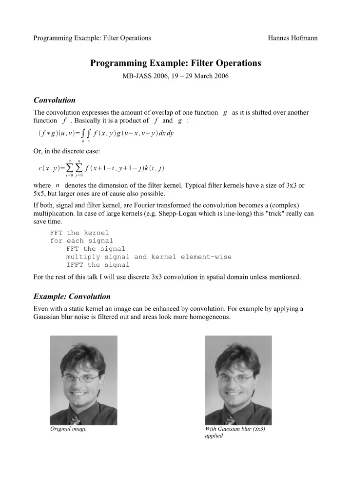
Even with a static kernel an image can be enhanced by convolution. For example by applying a Gaussian blur noise is filtered out and areas look more homogeneous.

Original image With Gaussian blur (3x3) applied

Programming Example: Filter Operations Hannes Hofmann Furthermore one can extract valuable information out of images, e.g. edge information.

Border Conditions

For each pixel we compute we need the values of the neighbouring pixels. For the border pixels not all neighbours exist, so we must define what values we will use in that case. The larger our kernel is the more pixels are missing.

–

Zeros Set all outer pixels to zero.

–

Clamping Use the value of the border pixel for all pixels that lie outside of the image.

–

Wrapping Take the value of the border pixel on the opposite side.

–

Anything else One may think of any other way to handle this problem, just make sure that you don't get undesired results.

Partitioning

The Local Store of our SPUs has only a capacity of 256 KB. Most real-world problems will not fit into that little storage. Furthermore we want to use more than just one SPU in parallel to reduce computation time. That is why we have to divide our problem into several smaller ones. Of course this implies an overhead and you have to decide if it's worth the effort. Each data block has its own borders e.g., so you may have to transfer more input date onto the SPUs than you get as

• result. And what happens if one subtask is much faster than another one? It would be a pitty if 7 out
• f 8 SPUs stall because they are waiting for the other one to finish.
• 1

1

• 1

2

• 2

1

• 1

1 2 1

• 1
• 2

Original image With horizontal Sobel With vertical Sobel

Programming Example: Filter Operations Hannes Hofmann

Partitioning: Strategies

One partitioning strategy that is known from DSPs is the pipeline model. The problem is divided into several subsequent sub-problems. Each of these is then assigned to one SPU that solves it and sends its results to the next SPU. Typically you don't want to do that on the Cell because you have to make sure that each stage of the pipeline takes approx. Equally long to avoid stalls.. A model that better fits to the CBEA is a static partitioning of the task. Basically you divide your input (or output) data into N blocks and send one to each of your SPUs, wait for all the results and send the next blocks. That way you can be sure that every SPU has about the same amount of work. In the case that you want some SPUs to do a different task you will run into troubles again, so you may want to use a more flexible scheduling algorithm. For example an SPU signals the PPU when it has finished its task and the PPU then gives the next workload to it. IBM has also introduced an advanced programming model called the microtask model in which the compiler assists the programmer in partitioning. Every block in the code is a microtask and as many mircotask as possible make an SPU task.

Scalar Code

The scalar convolution code is fairly simple. Just iterate over all pixels and sum up the products of all neighbours and the corresponding kernel element: for each line for each column as col for (k=0; k<3; ++k) {

• ut[line][col] += in[line][col+k] * kern[k]
• ut[line][col] += in[line+1][col+k] * kern[k+3]
• ut[line][col] += in[line+2][col+k] * kern[k+6]

} Note: the input image is larger than the output image here (see Border Conditions).

3x3 Convolution from IBM's sample library

The scalar code performs very bad on the Cell hardware, because it benefits from none of its performance improving features. Fortunately IBM supplies us with an optimized convolution that exploits the architcture. void _conv3x3_1f (const float *in[3], float *out, const vec_float4 m[9], int w) { // init local variables const vec_float4 *in0 = (const vec_float4 *)in[0]; // ... in2 vec_float4 m00 = m[0]; // ... m08 // pre-process // init some pointers to handle left border (_CLAMP_CONV, // _WRAP_CONV)

Programming Example: Filter Operations Hannes Hofmann // process the line for (i0=0, i1=1, i2=2, i3=3, i4=4; i0<(w>>2)-4; i0+=4, i1+=4, i2+=4, i3+=4, i4+=4) { res = resu = resuu = resuuu = VEC_SPLAT_F32(0.0f); _GET_SCANLINE_x4(p0, in0[i0], in0[i1], in0[i2], in0[i3], in0[i4]); _CONV3_1f(m00, m01, m02); _GET_SCANLINE_x4(p1, in1[i0], in1[i1], in1[i2], in1[i3], in1[i4]); _CONV3_1f(m03, m04, m05); _GET_SCANLINE_x4(p2, in2[i0], in2[i1], in2[i2], in2[i3], in2[i4]); _CONV3_1f(m06, m07, m08); vout[i0] = res; vout[i1] = resu; vout[i2] = resuu; vout[i3] = resuuu; } // process line // post-process // right border } At first some local variables are initialized. Those *u, *uu and *uuu variables have the same semantics as prev, curr and next, but are used to unroll the computation by a factor of 4 #define _GET_SCANLINE_x4(_p, _a, _b, _c, _d, _e) \ prev = _p; \ curr = prevu = _a; \ next = curru = prevuu = _b; \ nextu = curruu = prevuuu = _c; \ nextuu = curruuu = _p = _d; \ nextuuu = _e

4 36 1 1 5 7 9 11 4 7 1 1 6 9 9 8 1 3 3 7

in[0]=in0

prev curr, prevu next curru, prevuu nextuu curruuu nextu, curruu, prevuuu nextuuu

Programming Example: Filter Operations Hannes Hofmann _CONV3_1f is just a helper macro that calls others. #define _CONV3_1f(_m0, _m1, _m2) \ _GET_x4(prev, curr, left, left_shuf); \ _GET_x4(curr, next, right, right_shuf); \ _CALC_PIXELS_1f_x4(left, _m0, res); \ _CALC_PIXELS_1f_x4(curr, _m1, res); \ _CALC_PIXELS_1f_x4(right, _m2, res) Now it's time to visit the neighbours. shuf is a shuffle left or right by one pixel. #define _GET_x4(_a, _b, _c, _shuf) \ _c = vec_perm(_a, _b, _shuf); \ _c##u = vec_perm(_a##u, _b##u, _shuf); \ _c##uu = vec_perm(_a##uu, _b##uu, _shuf); \ _c##uuu = vec_perm(_a##uuu, _b##uuu, _shuf) And finally: work! Now the products are computed and accumulated. #define _CALC_PIXELS_1f_x4(_a, _b, _c) \ _c = vec_madd(_a, _b, _c); \ _c##u = vec_madd(_a##u, _b, _c##u); \ _c##uu = vec_madd(_a##uu, _b, _c##uu); \ _c##uuu = vec_madd(_a##uuu, _b, _c##uuu) The engineers at IBM did several optimizations of the scalar code.

• 1. Vectorization to exploit SIMD

By using the left and right variables in addition to the curr vector 4 pixels can be computed at the same time. All arithmetic instructions work on vectors of 4 floats (vec_madd). The possible speedup thereof is 4.

• 2. Loop-unrolling to avoid stalls

Those *u, *uu and *uuu variables allow the compiler to do a better scheduling of arithmetic and Load/Store/Shuffle operations on the two pipelines. This can improve the dual issue rate and reduce stalls. Another specialty of IBM's code is that it runs on VMX and SPU, just by switching the compiler.

5 7 9 11 in0 left, leftu, 1 5 7 9 7 9 11 4 right, rightu, // in scalar terms: res += left * m0 + curr * m1 + right * m2 curr

Programming Example: Filter Operations Hannes Hofmann

Approximate Register Usage

In case of a 3x3 convolution it is sufficient to have 35 registers available. As we have 128 of them there is quite a lot of room for the compiler to do further loop unrolling or other optimizations. If we increase the kernel size to 9x9 we need much more registers because we have need prev and next permutations of 1, 2 and 3 pixels. In IBM's implementation only one line of the kernel is kept in registers, so we have a total of about 55 registers used. Here we have also room for improvements, for example prefetching of the next kernel line.

Performance

The optimized implementation computes 16 pixels, each multiplied with one kernel row, in one

• iteration. 12 vector multiply-add and 8 vector permute operations are needed for that. For a 16

pixels convolved with a whole 3x3 kernel it takes 36 vec_madd and 24 vec_perm operations. The scalar version from the beginning needs 16*9=144 operations for the same task. I assume we do have a fused multiply-add operation to make a fair comparison. Furthermore Load/Store operations are not taken into account. Taking the vectorization into account we expect a speedup by a factor of 4. The optimized version should take no more than 144/4=36 operations. It is not very surprising that we need exactly that much arithmetic operations. But we also need permute operations. So the full speedup can only be gained if these are for free. In case of the Cell and a good compiler they in fact are, as they are on the other pipeline.

Example: Static Partitioning

As an example of a partitioning strategy a static approach will be shown here. The PPU divides the input and output images into NUM_SPUS blocks and gives one block to each SPU. The input image has to be larger than the output to avoid border conditions and for the indizes to be correct. This might be done in a preprocessing step on the PPU. int main(int argc, char *argv[]) { float *in, *out; int h; int part_h = h/NUM_SPUS; for (i=0; i<NUM_SPUS; i++) { ctx.in = in+i*part_h*w; ctx.h = part_h; ctx.w = w; ctx.out = out+i*part_h*w; ids[i] = spe_create_thread(0, &spu_conv, &ctx, NULL,

• 1, 0);

} for (i=0; i<NUM_SPUS; i++) { spe_wait(ids[i], &status, 0); } return (0); }

Programming Example: Filter Operations Hannes Hofmann

Example: Double Buffering

Let's assume that the Local Store is too small to hold all of our data, what quite realistic. Naivly we would fetch some data, process it and write back the result. This would be really imperformant, because we have no cache mechanism and every access to main memory via DMA has a latency hundrets or thousands of cycles during which the SPU would be idle. To avoid such stalls we will use double buffering. That means fetching data in advance (into a second buffer) to have it ready when it's needed. On the SPU side we need to do some initalizations first. That includes splating of the kernel into vectors and fetching the context containing the addresses of the data to process. int main(unsigned long long speid, unsigned long long argv) { volatile ctx_t ctx; volatile float in[3][MAX_LINE_W]; float out[MAX_LINE_W]; const float *ptrs[3]; float *kern = {1, 2, 1, 0, 0, 0, -1, -2, -1}; vec_float4 mask[9]; int next_tag, tag = 0; spu_writech(MFC_WrTagMask, 1 << 0); spu_mfcdma32((void *)(&ctx), (unsigned int)argv, sizeof(ctx_t), 0, MFC_GET_CMD); spu_mfcstat(2); for (j = 0; j < 9; j++) mask[j] = splat_float(kern[j]); After that we process the data using a double buffering algorithm. Therefore we prefetch the first lines and initialize the line pointers so we can start processing our image. // prefetch 3 lines spu_mfcdma32((void *)(in[0]), (unsigned int)(ctx.in), ctx.w*sizeof(float), tag, MFC_GET_CMD); // no increment of ctx.in -> clamping spu_mfcdma32((void *)(in[1]), (unsigned int)(ctx.in), ctx.w*sizeof(float), tag, MFC_GET_CMD); ctx.in += ctx.w; spu_mfcdma32((void *)(in[2]), (unsigned int)(ctx.in), ctx.w*sizeof(float), tag, MFC_GET_CMD); ctx.in += ctx.w; ptrs[0] = (const float *)(in[0]); ptrs[1] = (const float *)(in[1]); ptrs[2] = (const float *)(in[2]); In the main loop we start a DMA transfer to prefetch one line for the next iteration while we process the current one. Finally the result is written back to main memory and the line pointers are set to the next line.. for (y=3; y<ctx.h+1; y++) { next_tag = tag^1;

Programming Example: Filter Operations Hannes Hofmann // prefetch next line ++inBuf; if (inBuf >= 4) { inBuf = 0; } spu_mfcdma32((void *)(in[inBuf]), (unsigned int) (ctx.in), ctx.w*sizeof(float), next_tag, MFC_GETB_CMD); ctx.in += ctx.w; // wait for previous get (and put) spu_writech(MFC_WrTagMask, 1 << tag); (void)spu_mfcstat(2); // process line conv3x3_1f(ptrs, out[tag], mask, ctx.w); // write result back spu_mfcdma32((void *)(out[tag]), (unsigned int) (ctx.out), ctx.w*sizeof(float), tag, MFC_PUT_CMD); ctx.out += ctx.w; // next line ptrs[0] = ptrs[1]; ptrs[1] = ptrs[2]; ptrs[2] = (const float *) in[inBuf]; tag = next_tag; } At the very end we need to process the last line that was prefetched in the last loop iteration! The code is not shown here as it is the same as inside the main loop except of the missing prefetch. // process last line // wait for its results to be written return (0); } /* main */

References

IBM Cell SDK Sample Library (cell-sdk-lib-samples-1.0.1.tar.bz2)