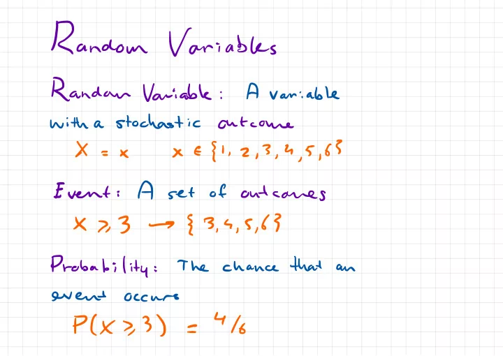
Event A of outcomes set : , 5,6 } { 7,3 X 3. s - - PowerPoint PPT Presentation

event
SMART_READER_LITE
LIVE PREVIEW

Event A of outcomes set : , 5,6 } { 7,3 X 3. s - - PowerPoint PPT Presentation

Random Variables Random A Variable variable : stochastic with outcome a E { , 63 2,3 4,5 1 = , , Event A of outcomes set : , 5,6 } { 7,3 X 3. s Probability that The chance an : event occurs 4/6 PCX


slide-1
SLIDE 1

Random

Variables Random Variable : A variable with a stochastic
  • utcome
= × × E { 1 , 2,3 , 4,5 , 63

Event

: A set
  • f
  • utcomes
X 7,3 { 3. s , 5,6 } Probability : The chance that an event
  • ccurs
PCX >, 3) = 4/6
slide-2
SLIDE 2 Distributions A distribution maps
  • utcomes
to probabilities P(X=x ) = 116 Commonly used (
  • r
abused ) shorthand ; Pc x ) P(X=x )
slide-3
SLIDE 3 Condition

'al

Probabilities joint Probability PC A. B ) :-. Plan 13 ) pp Events Conditional Probability P( Al B) :-. PC A. B) PC B)
slide-4
SLIDE 4

Sum

Rule General Case 0.4 0,5 t 0,6
  • 0.4
= 0.7 P (

Au

B ) =PLA ) +

PCB

)
  • PCA
, B) p p P Either a man Is a man Has short hair
  • r
has short hair 0,5 0.6 Marginal Corrolaiiies f P (A) = [ P(X=x ) P(4=y)={P(4=y ,X=x )

:X

e A T T ' T Events Rand uw
  • utcome
slide-5
SLIDE 5

Bayes

. Rule Pl Al B) = Pla ,R )
  • PC B)
Product Rule .

PGA

, B) = P ( AIB ) PCB ) = PCBIA ) PCA ) Bayes ' Rule PCAIB ) = Pl
  • A. B )
PCB ) = PLBIA ) Pla ) PC B)
slide-6
SLIDE 6 Example Event A :-( Prior You have a rare disease P( A) =
  • ooo:|
PGA ) = 0.9999 B : Test for disease is

positive

a as
  • 0.0001
Livelihood PCB 1 A) = a qa PIBIAIPIA )= gain 0.004 ( P ( Bl
  • A)
= 0.01 P( B. A) PGA ) a
  • .O
, PIB ) = PIBIAIPIA )tPlB) Question : What is

PCAIB

) ? PHA ) p( Al B) = Pl Bt A) Pla ) '
  • .
  • ,
  • =
  • =
  • .cl
PC B ) 0.01+0.0001
slide-7
SLIDE 7 Probability Densities Suppose that X is a continuous variable then P(X=x ) is for any
  • utcome
× f
  • utcome
X~ Normal 10,1 ) p(X=n ) =
  • pl3sXs4
) to a Define density function event P( x
  • 8s×<
x +8 ) pxcxs = him . 8
  • 28
slide-8
SLIDE 8 Probability Space ( R , F , P ) R Sample space ( set
  • f
possible
  • utcomes
) F Set
  • f
events ( every possible subet
  • f
the sample space ) P Probability measure g Event p Probability P : F [
  • , D
P ( Y E ;) = ? P ( Ei ) P ( ¢ ) =o (Empty set when {

Eil

disjoint has pvebo ) P ( R ) = 1 1 sample space has prob 1 )
slide-9
SLIDE 9 Examples
  • f
Reference Measures ( not probalitu ? Lebesgue Measure : µ( [ a ,b ] ) = b- a ( Width
  • f
interval ) Counting

Measure

: µ ( { x ;3¥ ) =

@

( Number
  • f
elements ) Product Measure : µ ( E ) = µ , IE , ) µ{ E . ) ( Cartesian Product ) E := ( E , , Ez )
slide-10
SLIDE 10 Definition
  • f
Probability Measure g probability measure g Differential
  • f
the net PCA ) :=

e a pyx ) dµc× , measure 4 4 \ Density Event Outcome function Machine Learning Notation ×=x P ( A) = |a pcx ) dx T Ref measure implied
slide-11
SLIDE 11 Expected Values E [ X ) := / x pcx ) dx X~ pcx ) . . . @ Implied by C 1 Statistician defines Conditional Expectation this first E[ f ( x. 4) I 4=y ]

:=

) f ( x. g)

pay

dx T Observed
  • data
Expectation w.int . a different distribution Eacx , [ f ( x ) ] = / fix > qcx ) dx T some dist qcx )
slide-12
SLIDE 12 Central problem in this course e- Quantity
  • f

Epcxiy

)[ fk , y ) ] interest Things we do www. (

Thitngs

we don't know Examples Self . driving Cars Diagnosis y Past trajectory Symptoms × Future trajectory Condition f Will pedestrian cross ? Treatment Outcome
slide-13
SLIDE 13 Example : Biased Coins X ~ Beta ( a , B) Bias × E [ 0,1 ] Yn ~ Bernoulli ( × ) ×=° 's ' coin is unbiased x=o always tails n = I , . . . , N × = i always heads Banes Rule yn= {

g

tails heads p ( X 14 , = y , , . . . ,4µ=yn ) Posterior Likelihood Prior = p ( 4 , = y , , . . . , YN = yn 1 X ) p ( X ) PCY , = y . , . . . , Uµ= yn , ) Marginal Likelihood
slide-14
SLIDE 14 Pinion Beta " ' " ' ' ' ¥-1,1 I I . a
  • i
p
  • l
Betak

;qp7=

× ( i
  • xs
BC 0,137
  • BIQB )
= P( a) 171137 co bur p
  • 11
  • × )
Parameters 176+13 ) Likelihood yi , ... ,bH µ ply , :n1× ) =

II.

plynlx )

¥Yates

, are piyn '× ) =

{

x yn=i = ×Yn(
  • i. XYT
" ( l
  • x )
yn=o
slide-15
SLIDE 15 g does depend
  • n
× Conjngacy

Plx

I yi ) =

ply

, :µ,×7 a ply , :µ,× )
  • Plyiin
) \ does not depend
  • h
× P ( yi :µ,× ) = pk ) ply , :m lx ) µ at B- 1 n yn ( l
  • yn
) = 1- × ( 1
  • × )
× ( l
  • X
\ 1310,131 nil = ,
  • III. but
to
  • 1
, , .nl#..tynHB . 1
  • n
BGIB ) ( Number
  • f
(^ Number
  • f
Sufficient heads in tails in statistics
  • N
trials N trials
slide-16
SLIDE 16 Conjngacy Plx I yi ) = ply , :µ,×7 a ply , :µ,×7
  • plyiin
) P ( Yi ,× ) = pk ) ply , :m lx ) N = 1

xo

"a . xsp "MxYn( , .× , "
  • 9
" B( a ,M n= , N £

:[

ynto = 1 ×l£IYnlta . ' , ,

.nl?Ea.ynDtB.ln=g=

  • B( a ,p7
=

=D

  • 1
N

15=1

, " Ya + ' =p , ,3,×£' (
  • i. xp
"

.tk#lBe+acx;a.B

) BA ,B )
slide-17
SLIDE 17 Doesn't depend
  • n
X Conjugate f Depends
  • n
× d ply , :n , × ) = BC I. B ) Betak;I , F) Bla , B) = plyi :u ) PCX I yi ) Posterior pcxiyi :n ) = Beta / x ; Q , F ) H E = . [ ynto Marginal Likelihood nu ply , :u ) = B(I,pif B = & , .li
  • yn )
+ 13 B( a ,B )
slide-18
SLIDE 18 Predictive Distribution Joint

probability

  • f
next trial and coin bias
  • p
( yµ+ , 1 Yi :X , ) = | dx plymti , × 1 Yi :X ,) =

/

dx p ( yµ+ , 1×1 pklyi :N ) = Epcxiy , :* ) [ plyntilxl ) Weighted Coin Example ( Exercise )
slide-19
SLIDE 19 Why is Bayesian Inference Hard ? Example : Mixture
  • f
Gaussians Center µw ~ Normal ( 0,1 ) he 1 , ... , K Width 6h ~ Gamma 11,1 ) Cluster Z in ~ Discrete ( 11k , ... , 1 He ) n = 1 , . . . ,N Assignment yn 1 Zn=h ~ Normal ( Mh ,6u ) Marginal Likelihood µ K K K PC yi :N ) =) die , :,<d6 , , ,<d7 , :µP( Yi :n ,7i

.nl/Ui:k,6i:k

)