evaluation of deterministic truncation of monte carlo
play

Evaluation of Deterministic Truncation of Monte Carlo (DTMC) - PDF document

Transactions of the Korean Nuclear Society Virtual Spring Meeting July 9-10, 2020 Evaluation of Deterministic Truncation of Monte Carlo (DTMC) Solutions with Partial Currents Fine-Mesh Finite Difference Formulations Inhyung Kim a and Yonghee Kim


  1. Transactions of the Korean Nuclear Society Virtual Spring Meeting July 9-10, 2020 Evaluation of Deterministic Truncation of Monte Carlo (DTMC) Solutions with Partial Currents Fine-Mesh Finite Difference Formulations Inhyung Kim a and Yonghee Kim a * a Nuclear and Quantum Engineering, Korea Advanced Institute of Science and Technology (KAIST), 291 Daejak-ro, Yu-seong-gu, Daejeon 34141, Republic of Korea, * Corresponding author: yongheekim@kaist.ac.kr 1. Introduction source convergence; thus, it can decrease the computing A deterministic truncation of Monte Carlo (DTMC) time of the inactive cycles. Meanwhile, the DTMC solution method is one of numerical schemes developed solutions can provide accurate solutions equivalent to for the acceleration of a Monte Carlo (MC) simulation the high-fidelity MC solutions, while having lower and the variance reduction of the solutions. The DTMC statistical uncertainties because the deterministic method proceeds a statistical treatment of the computation is rather free from the random process. deterministic solutions truncated by the fine mesh finite difference (FMFD) method in the MC calculation. The DTMC method can significantly decrease the computing time by accelerating the convergence of the fission source distribution (FSD) during inactive cycles, and also decrease the statistical errors of the reactor parameters from the early active cycles [1,2]. The DTMC method has adopted the FMFD method to truncate the MC solutions. However, in this study, the partial current based FMFD (pFMFD) method is applied to improve the numerical stability of the DTMC method. Furthermore, a decoupled DTMC scheme is newly attempted to get rid of the possible bias in the FMFD-assisted MC solutions. In this paper, the numerical performance of the pDTMC method is characterized and compared to the standard MC method in a SMR problem. The multiplication factor, pin power Fig. 1. Diagram of the FMFD and DTMC methods distribution, and its statistical uncertainties are evaluated depending on the cycle accumulation length for the generation of the FMFD parameters. Last, the computing time and figure-of-merit (FOM) are also assessed. 2. Methods and Results 
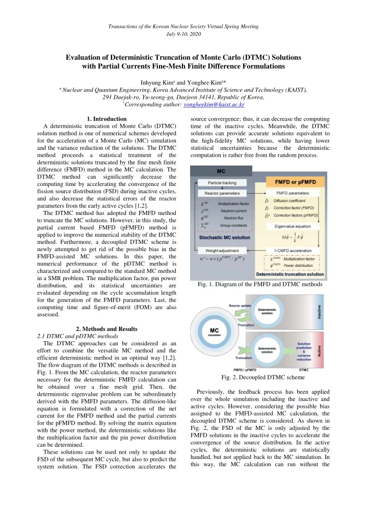
2.1 DTMC and pDTMC methods The DTMC approaches can be considered as an effort to combine the versatile MC method and the efficient deterministic method in an optimal way [1,2]. The flow diagram of the DTMC methods is described in Fig. 1. From the MC calculation, the reactor parameters Fig. 2. Decoupled DTMC scheme necessary for the deterministic FMFD calculation can be obtained over a fine mesh grid. Then, the Previously, the feedback process has been applied deterministic eigenvalue problem can be subordinately over the whole simulation including the inactive and derived with the FMFD parameters. The diffusion-like active cycles. However, considering the possible bias equation is formulated with a correction of the net assigned to the FMFD-assisted MC calculation, the current for the FMFD method and the partial currents decoupled DTMC scheme is considered. As shown in for the pFMFD method. By solving the matrix equation Fig. 2, the FSD of the MC is only adjusted by the with the power method, the deterministic solutions like FMFD solutions in the inactive cycles to accelerate the the multiplication factor and the pin power distribution convergence of the source distribution. In the active can be determined. cycles, the deterministic solutions are statistically These solutions can be used not only to update the handled, but not applied back to the MC simulation. In FSD of the subsequent MC cycle, but also to predict the this way, the MC calculation can run without the system solution. The FSD correction accelerates the

  2. Transactions of the Korean Nuclear Society Virtual Spring Meeting July 9-10, 2020 deterministic contamination, and the unbiased MC additional acceleration [1,5]. Furthermore, the one-node solutions can be truncated. CMFD acceleration scheme has been also considered to speed up the deterministic FMFD calculation [2]. The 2.2 FMFD and pFMFD methods details will not be discussed in this paper. Given the FMFD parameters generated from the MC simulation, the one-group diffusion-like neutron balance 2.4 Apparent and real standard deviations equation can be expressed on the node i as In the MC calculation, the reactor parameters should be statistically treated to understand the average 1  1         i i A J ( J ) , (1)   behavior. The parameters are averaged over cycles, and s s 1/2 s 1/2 a i f i V k  s i j k , , i eff its reliability is estimated by the standard deviation. where s indicates the surface index, V is the node However, due to the cycle correlation, the standard  volume, A is the node surface area, is the deviation estimated from a single MC run, so called a absorption cross section, J is the net current,  is the apparent standard deviation ( σ a ), could be under- estimated. Therefore, the real standard deviation ( σ r )   neutron flux, k is the multiplication factor, and eff f should be calculated by accounting for numerous is the number of neutrons per fission reaction times the independent batches with the different random seeds. fission cross section. The FMFD parameters are The apparent standard deviation (SD) of the accumulated over several contiguous cycles to be stable multiplication factor at the specific batch b can be and reliable. calculated by In the FMFD method [3], the net current in the x - N 1   c direction can be written as    b b b 2 (10) ( k k ) a c ˆ          N ( N 1) J D ( ) D ( ) , (2)  c 1 c c      i 1/2 i 1/2 i 1 i i 1/2 i 1 i where c is the active cycle index, b is the batch index, 2 D D   i 1 i where D , D is the diffusion b  N is the number of active cycles, k is the   i 1/2 ( D D ) c c  i 1 i i multiplication factor at the cycle c of the batch b , and ˆ coefficient,  is the node size, and D  is the i 1/2 N 1  c  b b k k . (11) correction factor: c N      c 1 MC MC MC c J D ( ) ˆ     i 1/2 i 1/2 i 1 i D . (3) In the meantime, the real SD can be calculated with  1/2    i MC MC  i 1 i the amount of the independent batches. On the other hand, in the pFMFD method [3], the two N 1   b    partial currents at the interface surface are preserved, * b 2 ( k k ) (12) r N 1 and thus the net current can be written in terms of the  b 1 b partial currents: where N is the number of batches, and b     J J J (4)    N i 1/2 i 1/2 i 1/2 1  b  * b k k (13) where the partial currents can be presented as N  b 1 b 1 ˆ          J D ( ) D , (5) For the power distribution, the apparent and real SDs     i 1/2 i 1/2 i 1 i i 1/2 i 2 are calculated at each node similarly to Eqs. (10) and 1 ˆ          (12). Therefore, the apparent SD is estimated by J D ( ) D (6)      i 1/2 i 1/2 i 1 i i 1/2 i 1 2 N 1   c    b b b 2 Then, the net current can be rewritten by ( p p ) (14) a i j k ,( , , ) ( , , ) i j k c i j k ,( , , ) N ( N 1) ˆ ˆ             c 1 c c J D ( ) D D (7)       i 1/2 i 1/2 i 1 i i 1/2 i i 1/2 i 1 and the real SD is estimated by ˆ D  where is the correction factors:  i 1/2 N 1   b         * b 2 , MC MC MC ( p p ) (15) J 0.5 D ( ) ˆ      r i j k ,( , , ) ( , , ) i j k ( , , ) i j k i 1/2 i 1/2 i 1 i N 1 D , and (8)    b 1 i 1/2 b MC i b where p is the normalized power value at the      , MC MC MC c i j k ,( , , ) J 0.5 D ( ) ˆ      i 1/2 i 1/2 i 1 i D (9) node ( i,j,k ) at the cycle c of the batch b ,   i 1/2 MC  i 1 N 1  c  b b p p (16) The two correction factors at each interface surface ( , , ) ,( , , ) i j k c i j k N  c 1 would consolidate the nodal equivalence with one more c and degree of freedom contrary to the FMFD method [4]. N 2.3 m-PRUP and 1-CMFD methods 1  b  * b p p (17) To enhance the numerical stability, the modified ( , , ) i j k ( , , ) i j k N  b 1 b particle ramp-up (m-PRUP) method has been developed. Last, the node-wise SDs are averaged over the whole It can determine the inactive cycle size and the nodes: generation size in a systematic way and also provide

Download Presentation
Download Policy: The content available on the website is offered to you 'AS IS' for your personal information and use only. It cannot be commercialized, licensed, or distributed on other websites without prior consent from the author. To download a presentation, simply click this link. If you encounter any difficulties during the download process, it's possible that the publisher has removed the file from their server.

Recommend


More recommend