Estimation theory Parametric estimation Properties of estimators - PowerPoint PPT Presentation

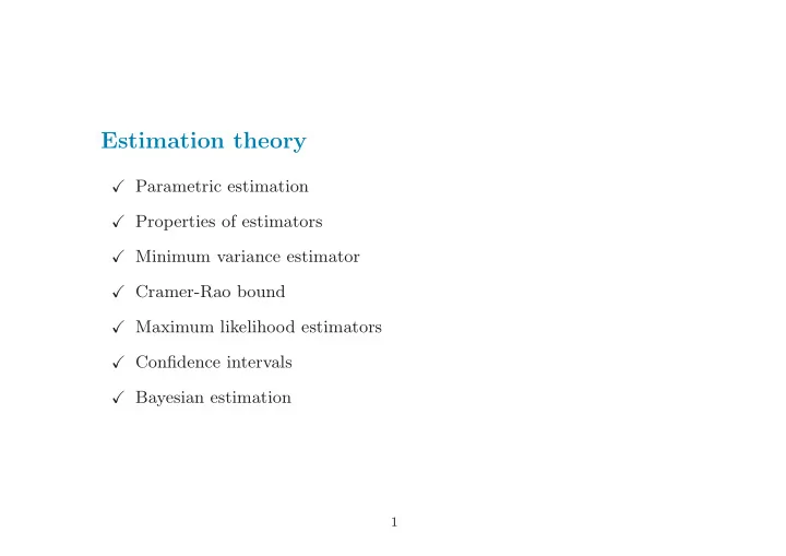
Estimation theory � Parametric estimation � Properties of estimators � Minimum variance estimator � Cramer-Rao bound � Maximum likelihood estimators � Confidence intervals � Bayesian estimation 1

Random Variables Let X be a scalar random variable (rv) X : Ω → R defined over the set of elementary events Ω. The notation X ∼ F X ( x ) , f X ( x ) denotes that: • F X ( x ) is the cumulative distribution function (cdf) of X F X ( x ) = P { X ≤ x } , ∀ x ∈ R • f X ( x ) is the probability density function (pdf) of X � x ∀ x ∈ R F X ( x ) = f X ( σ ) dσ, −∞ 2

Multivariate distributions Let X = ( X 1 , . . . , X n ) be a vector of rvs X : Ω → R n defined over Ω. The notation X ∼ F X ( x ) , f X ( x ) denotes that: • F X ( x ) is the joint cumulative distribution function (cdf) of X ∀ x = ( x 1 , . . . , x n ) ∈ R n F X ( x ) = P { X 1 ≤ x 1 , . . . , X n ≤ x n } , • f X ( x ) is the joint probability density function (pdf) of X � x 1 � x n ∀ x ∈ R n F X ( x ) = . . . f X ( σ 1 , . . . , σ n ) dσ 1 . . . dσ n , −∞ −∞ 3

Moments of a rv • First order moment ( mean ) � + ∞ m X = E [ X ] = x f X ( x ) dx −∞ • Second order moment ( variance ) � + ∞ ( x − m X ) 2 f X ( x ) dx σ 2 ( X − m X ) 2 � � X = Var( X ) = E = −∞ Example The normal or Gaussian pdf , denoted by N ( m, σ 2 ), is defined as − ( x − m ) 2 1 2 σ 2 √ f X ( x ) = e . 2 πσ It turns out that E [ X ] = m and Var( X ) = σ 2 . 4

Conditional distribution Bayes formula f X | Y ( x | y ) = f X,Y ( x, y ) f Y ( y ) One has: � + ∞ ⇒ f X ( x ) = f X | Y ( x | y ) f Y ( y ) dy −∞ ⇒ If X and Y are independent: f X | Y ( x | y ) = f X ( x ) Definitions: � + ∞ • conditional mean: E [ X | Y ] = x f X | Y ( x | y ) dx −∞ � + ∞ ( x − E [ X | Y ]) 2 f X | Y ( x | y ) dx • conditional variance: = P X | Y −∞ 5

Gaussian conditional distribution Let X and Y Gaussian rvs such that: E [ X ] = m X E [ Y ] = m Y ′          X − m X  X − m X R X R XY  = E      R ′ Y − m Y Y − m Y R Y XY It turns out that: m X + R XY R − 1 E [ X | Y ] = Y ( Y − m Y ) R X − R XY R − 1 Y R ′ = P X | Y XY 6

Estimation problems Problem. Estimate the value of θ ∈ R p , using an observation y of the rv Y ∈ R n . Two different settings: a. Parametric estimation The pdf of Y depends on the unknown parameter θ b. Bayesian estimation The unknown θ is a random variable 7

Parametric estimation problem • The cdf and pdf of Y depend on the unknown parameter vector θ , Y ∼ F θ Y ( x ) , f θ Y ( x ) • Θ ⊆ R p denotes the parameter space , i.e., the set of values which θ can take • Y ⊆ R n denotes the observation space , to which belongs the rv Y 8

Parametric estimator The parametric estimation problem consists in finding θ on the basis of an observation y of the rv Y . Definition 1 An estimator of the parameter θ is a function T : Y − → Θ Given the estimator T ( · ), if one observes, y , then the estimate of θ is ˆ θ = T ( y ). There are infinite possible estimators (all the functions of y !). Therefore, it is crucial to establish a criterion to assess the quality of an estimator. 9

Unbiased estimator Definition 2 An estimator T ( · ) of the parameter θ is unbiased (or correct ) if E θ [ T ( · )] = θ , ∀ θ ∈ Θ . unbiased biased θ Pdf of two estimators T ( · ) 10

Examples • Let Y 1 , . . . , Y n be identically distributed rvs, with mean m . The sample mean n Y = 1 ¯ � Y i n i =1 is an unbiased estimator of m . Indeed, n � ¯ = 1 � � E Y E [ Y i ] = m n i =1 • Let Y 1 , . . . , Y n be independent identically distributed (i.i.d.) rvs, with variance σ 2 . The sample variance n 1 S 2 = � ( Y i − ¯ Y ) 2 n − 1 i =1 is an unbiased estimator of σ 2 . 11

Consistent estimator Definition 3 Let { Y i } ∞ i =1 be a sequence of rvs. The sequence of estimators T n = T n ( Y 1 , . . . , Y n ) is said to be consistent if T n converges to θ in probability for all θ ∈ Θ , i.e. n →∞ P {� T n − θ � > ε } = 0 lim ∀ ε > 0 ∀ θ ∈ Θ , , n = 500 n = 100 n = 50 n = 20 θ A sequence of consistent estimators T n ( · ) 12

Example Let Y 1 , . . . , Y n be independent rvs with mean m and finite variance. The sample mean n Y = 1 ¯ � Y i n i =1 is a consistent estimator of m , thanks to the next result. Theorem 1 (Law of large numbers) Let { Y i } ∞ i =1 be a sequence of independent rvs with mean m and finite variance. Then, the sample mean ¯ Y converges to m in probability. 13

A suffcient condition for consistency Theorem 2 Let ˆ θ n = T n ( y ) be a sequence of unbiased estimators of θ ∈ R , based on the realization y ∈ R n of the n -dimensional rv Y , i.e.: E θ [ T n ( y )] = θ, ∀ n, ∀ θ ∈ Θ . If n → + ∞ E θ � ( T n ( y ) − θ ) 2 � lim = 0 , then, the sequence of estimators T n ( · ) is consistent. Example. Let Y 1 , . . . , Y n be independent rvs with mean m and variance σ 2 . We know that the sample mean ¯ Y is an unbiased estimate of m . Moreover, it turns out that Y ) = σ 2 Var( ¯ n Therefore, the sample mean is a consistent estimator of the mean. 14

Mean square error Consider an estimator T ( · ) of the scalar parameter θ . Definition 4 We define mean square error (MSE) of T ( · ) , ( T ( Y ) − θ ) 2 � E θ � If the estimator T ( · ) is unbiased, the mean square error corresponds to the variance of the estimation error T ( Y ) − θ . Definition 5 Given two estimators T 1 ( · ) and T 2 ( · ) of θ , T 1 ( · ) is better than T 2 ( · ) if ( T 1 ( Y ) − θ ) 2 � ( T 2 ( Y ) − θ ) 2 � E θ � ≤ E θ � ∀ θ ∈ Θ , If we restrict our attention to unbiased estimators, we are interested to the one with the least MSE for any value of θ (notice that it may not exist). 15

Minimum variance unbiased estimator Definition 6 An unbiased estimator T ∗ ( · ) of θ is UMVUE (Uniformly Minimum Variance Unbiased Estimator) if E θ � ( T ∗ ( Y ) − θ ) 2 � ≤ E θ � ( T ( Y ) − θ ) 2 � ∀ θ ∈ Θ , for any unbiased estimator T ( · ) of θ . UMVUE θ 16

Minimum variance linear estimator Let us restrict our attention to the class of linear estimators n � a i ∈ R T ( x ) = a i x i , i =1 Definition 7 A linear unbiased estimator T ∗ ( · ) of the scalar parameter θ is said to be BLUE (Best Linear Unbiased Estimator) if E θ � ( T ∗ ( Y ) − θ ) 2 � ≤ E θ � ( T ( Y ) − θ ) 2 � ∀ θ ∈ Θ , for any linear unbiased estimator T ( · ) di θ . Example Let Y i be independent rvs with mean m and variance σ 2 i , i = 1 , . . . , n . n 1 1 ˆ � Y = Y i n σ 2 1 i � i =1 σ 2 i i =1 is the BLUE estimator of m . 17

Cramer-Rao bound The Cramer-Rao bound is a lower bound to the variance of any unbiased estimator of the parameter θ . Theorem 3 Let T ( · ) be an unbiased estimator of the scalar parameter θ , and let the observation space Y be independent on θ . Then (under some technical assumptions), E θ � ( T ( Y ) − θ ) 2 � ≥ [ I n ( θ )] − 1 �� ∂ ln f θ � 2 � Y ( Y ) where I n ( θ )= E θ ( Fisher information ). ∂θ Remark To compute I n ( θ ) one must know the actual value of θ ; therefore, the Cramer-Rao bound is usually unknown in practice. 18

Cramer-Rao bound For a parameter vector θ and any unbiased estimator T ( · ), one has ( T ( Y ) − θ ) ( T ( Y ) − θ ) ′ � ≥ [ I n ( θ )] − 1 E θ � (1) where �� ∂ ln f θ � ′ � ∂ ln f θ �� Y ( Y ) Y ( Y ) I n ( θ ) = E θ ∂θ ∂θ is the Fisher information matrix . The inequality in (1) is in matricial sense ( A ≥ B means that A − B is positive semidefinite). Definition 8 An unbiased estimator T ( · ) such that equality holds in (1) is said to be efficient . 19

Cramer-Rao bound If the rvs Y 1 , . . . , Y n are i.i.d. , it turns out that I n ( θ ) = nI 1 ( θ ) Hence, for fixed θ the Cramer-Rao bound decreases as 1 n with the size n of the data sample. Example Let Y 1 , . . . , Y n be i.i.d. rvs with mean m and variance σ 2 . Then n ≥ [ I n ( θ )] − 1 = [ I 1 ( θ )] − 1 �� ¯ = σ 2 � 2 � Y − m E n where ¯ Y denotes the sample mean. Moreover, if the rvs Y 1 , . . . , Y n are normally distributed, one has also I 1 ( θ )= 1 σ 2 . Since the Cramer-Rao bound is achieved, in the case of normal i.i.d rvs, the sample mean is an efficient estimator of the mean . 20

Maximum likelihood estimators Consider a rv Y ∼ f θ Y ( y ), and let y be an observation of Y . We define likelihood function , the function of θ (for fixed y ) L ( θ | y ) = f θ Y ( y ) We choose as estimate of θ the value of the parameter which maximises the likelihood of the observed event (this value depends on y !). Definition 9 A maximum likelihood estimator of the parameter θ is the estimator T ML ( x ) = arg max θ ∈ Θ L ( θ | x ) Remark The functions L ( θ | x ) and ln L ( θ | x ) achieve their maximum values for the same θ . In some cases is easier to find the maximum of ln L ( θ | x ) (exponential distributions). 21