
SLIDE 1
Empirical Methods in Natural Language Processing Lecture 4 Language Modeling (II): Smoothing and Back-Off
Philipp Koehn 17 January 2008
PK EMNLP 17 January 2008 1
Language Modeling Example
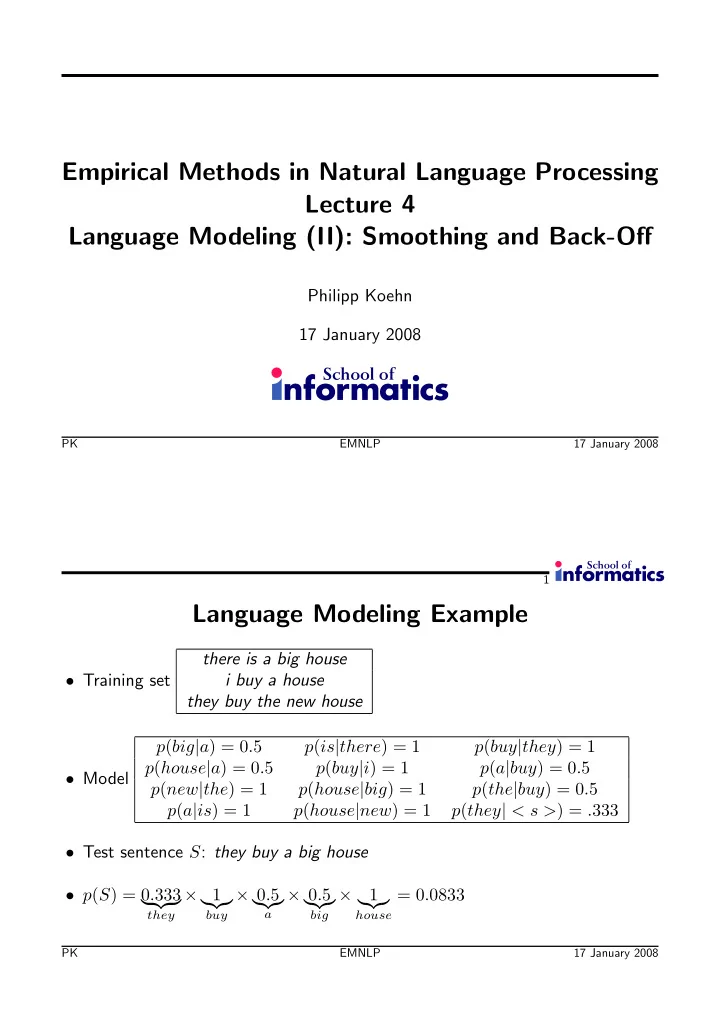
- Training set
there is a big house i buy a house they buy the new house
- Model
p(big|a) = 0.5 p(is|there) = 1 p(buy|they) = 1 p(house|a) = 0.5 p(buy|i) = 1 p(a|buy) = 0.5 p(new|the) = 1 p(house|big) = 1 p(the|buy) = 0.5 p(a|is) = 1 p(house|new) = 1 p(they| < s >) = .333
- Test sentence S: they buy a big house
- p(S) = 0.333
they
× 1
- buy
× 0.5
- a
× 0.5
- big
× 1
- house
= 0.0833
PK EMNLP 17 January 2008