economics 2 professor christina romer spring 2020
play

Economics 2 Professor Christina Romer Spring 2020 Professor David - PDF document

Economics 2 Professor Christina Romer Spring 2020 Professor David Romer LECTURE 21 FISCAL POLICY April 14, 2020 I. R EVIEW OF THE K EYNESIAN C ROSS D IAGRAM A. Determination of output in the short run B. What causes short-run fluctuations? C.


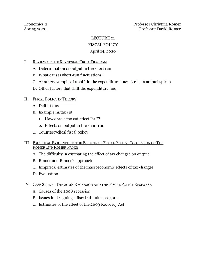
  1. Economics 2 Professor Christina Romer Spring 2020 Professor David Romer LECTURE 21 FISCAL POLICY April 14, 2020 I. R EVIEW OF THE K EYNESIAN C ROSS D IAGRAM A. Determination of output in the short run B. What causes short-run fluctuations? C. Another example of a shift in the expenditure line: A rise in animal spirits D. Other factors that shift the expenditure line II. F ISCAL P OLICY IN T HEORY A. Definitions B. Example: A tax cut 1. How does a tax cut affect PAE? 2. Effects on output in the short run C. Countercyclical fiscal policy III. E MPIRICAL E VIDENCE ON THE E FFECTS OF F ISCAL P OLICY : D ISCUSSION OF T HE R OMER AND R OMER P APER A. The difficulty in estimating the effect of tax changes on output B. Romer and Romer’s approach C. Empirical estimates of the macroeconomic effects of tax changes D. Evaluation IV. C ASE S TUDY : T HE 2008 R ECESSION AND THE F ISCAL P OLICY R ESPONSE A. Causes of the 2008 recession B. Issues in designing a fiscal stimulus program C. Estimates of the effect of the 2009 Recovery Act
  2. Economics 2 Christina Romer Spring 2020 David Romer L ECTURE 21 Fiscal Policy April 14, 2020

  3. Announcements • We have handed out Problem Set 5, Part 1. • It is due at 2 p.m. PDT on Thursday, April 16 th .

  4. I. R EVIEW OF THE K EYNESIAN C ROSS D IAGRAM

  5. Determination of Short-Run Output • Equilibrium condition: Y = PAE • Y is output and PAE is planned aggregate expenditure. • Output responds to demand in the short run. • Referred to as the 45-degree line.

  6. Determination of Short-Run Output PAE Y=PAE Y

  7. Determination of Short-Run Output (Continued) • Planned spending is a function of output: PAE = C + I p + G + NX • Where C depends on positively on Y, so PAE also depends positively on Y. • Referred to as the expenditure line.

  8. Determination of Short-Run Output PAE PAE Y

  9. Determination of Short-Run Output (Continued) • Short-run output is determined by the intersection of the 45-degree line and the expenditure line.

  10. Determination of Short-Run Output PAE Y=PAE PAE Y 1 Y Sometimes called the “Keynesian Cross” diagram.

  11. What Causes Short-Run Fluctuations? • Anything that shifts the expenditure line will cause output to change in the short run.

  12. Example: A Rise in Animal Spirits • Suppose that something causes firms throughout the economy to raise their expectations of the future MRP K . • This will make firms want to do more investment. • This will shift up the expenditure line.

  13. A Rise in Animal Spirits PAE Y=PAE PAE 2 PAE 1 Y 2 Y* Y The rise in Y is larger than the initial increase in PAE because of the multiplier effect.

  14. What Shifts the Expenditure Line? • A change in autonomous consumption (consumer confidence, wealth, uncertainty). • A change in firm’s expectations of future MRP K (animal spirits). • A change in the real interest rate. • A change in taxes or government purchases. • A change in net exports.

  15. Two Types of Macroeconomic Policy • Fiscal policy: Actions taken by the government to change the budget surplus. • Monetary policy: Actions taken by the central bank to affect nominal and real interest rates.

  16. II. F ISCAL P OLICY IN T HEORY

  17. Fiscal Policy Terminology • Government budget surplus: • Tax revenues − Government purchases (T−G) • Contractionary fiscal policy: Actions that increase the government budget surplus. • Will decrease PAE at a given level of Y. • Expansionary fiscal policy: Actions that decrease the government budget surplus. • Will increase PAE at a given level of Y.

  18. Federal Budget Surplus and the Bush Tax Cuts 3 2 1 Percent of GDP 0 1997 1998 1999 2000 2001 2002 2003 2004 2005 2006 -1 -2 -3 -4 Source: Congressional Budget Office.

  19. Short-Run Effects of a Tax Cut PAE Y=PAE PAE 2 PAE 1 Y 2 Y 1 Y (Y*)

  20. Substituting the Consumption Function into PAE C = C + c·(Y−T) PAE = C + I p + G + NX = C + c·(Y − T) + I p + G + NX = C + cY – cT + I p + G + NX = (C – cT + I p + G + NX) + cY PAE Intercept Term

  21. Combining the Effects of a Fall in Autonomous Consumption and a Tax Cut PAE Y=PAE PAE 1 ,PAE 3 PAE 2 PAE shifts back up (to PAE 3 ) because of the tax cut. PAE shifts down (to PAE 2 ) because of the fall in autonomous consumption. Y* Y

  22. Countercyclical Fiscal Policy • Deliberate changes in the budget surplus (through changes in taxes or government purchases) to try to counteract other factors likely to cause a short- run fluctuation.

  23. III. E MPIRICAL E VIDENCE ON THE E FFECTS OF F ISCAL P OLICY : D ISCUSSION OF THE R OMER AND R OMER P APER

  24. Difficulty in Estimating the Effect of Tax Changes • Some tax cuts are taken because output is falling. • Would not expect output to rise following these tax cuts. • This is an example of omitted variable bias . • A third variable (whatever is causing the recession) is driving both output and tax changes. • Positive effects of tax cuts will be underestimated.

  25. How do Romer and Romer try to deal with this difficulty? • Identify the motivation for the tax changes using narrative sources. • Read Congressional reports, Presidential speeches, Economic Report of the President . • Then limit the statistical analysis only to tax changes not taken in response to the state of the economy.

  26. Exogenous Tax Changes Source: Romer and Romer, “The Macroeconomic Effects of Tax Changes.”

  27. Specification • Δ Y is the percentage change in real GDP. • ΔT is the new measure of exogenous tax changes (as a percent of GDP). • The regression estimates the relationship between output growth and the contemporaneous and lagged values of tax changes. • We expect a negative relationship.

  28. Estimated Impact of a Tax Cut of 1% of GDP on Real GDP 5 4 Cumulative Impact (Percent) 3 2 1 0 -1 0 1 2 3 4 5 6 7 8 9 10 11 12 Quarters after the Tax Cut Source: Romer and Romer, “The Macroeconomic Effects of Tax Changes.”

  29. Evaluation • Do you trust the narrative sources? • Is narrative analysis reproducible? • Does this approach deal with omitted variable bias successfully?

  30. IV. C ASE S TUDY : T HE 2008 R ECESSION AND THE F ISCAL P OLICY R ESPONSE

  31. Source: Federal Reserve Bank of St. Louis, FRED. Case-Shiller House Price Index, January 2000 = 100 100 150 200 250 50 0 Jan-87 House Prices, 1987–2015 Jan-89 Jan-91 Jan-93 Jan-95 Jan-97 Jan-99 Jan-01 April 2006 Jan-03 Jan-05 Jan-07 Jan-09 Jan-11 Jan-13 Jan-15

  32. Effects of the Housing Bubble • Increased both I p and C, so raised PAE relative to what it otherwise would have been. • Some debate among economists about whether this increase in PAE counteracted other forces lowering PAE, or pushed Y above Y*. • Large increase in household debt.

  33. U.S. Household Debt Source: Mian and Sufi, “Consumers and the Economy, Part II: Household Debt and the Weak U.S. Recovery.”

  34. What happened when the bubble burst?

  35. Single-Family Housing Starts Source: Economic Report of the President , February 2010.

  36. Real Personal Consumption Expenditures November 2007 Source: FRED, Bureau of Economic Analysis.

  37. Source: http://www.housingviews.com.

  38. Credit Spreads during the Financial Crisis Source: Economic Report of the President , February 2010.

  39. Stock Prices during the Financial Crisis Source: Economic Report of the President , February 2010.

  40. What happened to PAE in 2008? • Decline in investment (particularly in housing) • Housing bust reduced expected future MRP K of housing (which is a kind of capital). • Financial crisis hurt animal spirits and made it hard for firms to get credit. • Decline in consumption • Housing bust and stock market decline destroyed wealth. • Financial crisis hurt consumer confidence and made it hard for households to get credit.

  41. Effect of the Housing Bust and the Financial Crisis on Output PAE Y=PAE PAE 1 PAE 2 Y 2 Y* Y

  42. Source: Federal Reserve Bank of St. Louis, FRED Percent Change (at an Annual Rate) -10.0 10.0 -8.0 -6.0 -4.0 -2.0 0.0 2.0 4.0 6.0 8.0 Percentage Change in Real GDP 2000-I 2001-I 2002-I 2003-I 2004-I 2005-I 2006-I 2007-I 2008-I 2009-I 2010-I 2011-I 2012-I 2013-I 2014-I 2015-I

  43. Issues in Designing the 2009 Fiscal Stimulus • How big should it be? • Need an estimate of how much PAE has shifted down. • Or, alternatively, how much Y would fall (and unemployment would rise) as a result of the decline in PAE. • Forecasts were much too optimistic early in the recession.

  44. Issues in Designing the 2009 Fiscal Stimulus • What should the composition be? • Different types of stimulus have different effects on PAE. • $100 billion increase in G will increase PAE by $100 billion; $100 billion of tax cuts will increase PAE by MPC·$100 billion. • Different types of stimulus affect the economy with different speeds.

  45. Fiscal Stimulus in the Recovery Act through August 2009 Source: CEA, “The Economic Impact of the ARRA of 2009, First Quarterly Report.”

Download Presentation
Download Policy: The content available on the website is offered to you 'AS IS' for your personal information and use only. It cannot be commercialized, licensed, or distributed on other websites without prior consent from the author. To download a presentation, simply click this link. If you encounter any difficulties during the download process, it's possible that the publisher has removed the file from their server.

Recommend


More recommend