ECON 950 Winter 2020 Prof. James MacKinnon 10. Performance of - PowerPoint PPT Presentation

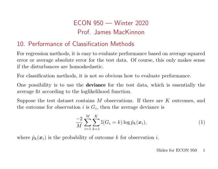
ECON 950 — Winter 2020 Prof. James MacKinnon 10. Performance of Classification Methods For regression methods, it is easy to evaluate performance based on average squared error or average absolute error for the test data. Of course, this only makes sense if the disturbances are homoskedastic. For classification methods, it is not so obvious how to evaluate performance. One possibility is to use the deviance for the test data, which is essentially the average fit according to the loglikelihood function. Suppose the test dataset contains M observations. If there are K outcomes, and the outcome for observation i is G i , then the average deviance is M K − 2 ∑ ∑ I ( G i = k ) log ˆ p k ( x i ) , (1) M i =1 k =1 where ˆ p k ( x i ) is the probability of outcome k for observation i . Slides for ECON 950 1

In the binary case, if we used a logit model (with or without regularization), the probability is either exp( X i ˆ β ) 1 or (2) . 1 + exp( X i ˆ 1 + exp( X i ˆ β ) β ) Thus the average deviance for the test data is M 1 β ) + 1 1 + exp X i ˆ X i ˆ ∑ ∑ ( − log (3) β . M M y i =1 i =1 Many classification methods do not give probabilities, however. They just classify each observation in the test set. Moreover, if we care about mistakes in classification, a criterion based on probabil- ities may not be what we want. Consider the binary case. Let 1 denote “a positive” and 0 denote “a negative.” For example, having a disease might be a 1, and not having it might be a 0. Slides for ECON 950 2

We may care much more about false negatives than false positives, so a criterion like deviance that weights them equally may not be appropriate. Four possible outcomes are: • True positive (TP) • True negative (TN) • False positive (FP) • False negative (FN) Then the true positive rate , or sensitivity , is TP TPR = (4) TP + FN , and the true negative rate , or specificity , is TN TNR = (5) TN + FP . In each case, the rate is the ratio of true positives (or negatives) to the total number of positives (or negatives) in the test set. Slides for ECON 950 3

There are many other ratios that we could calculate, such as the false positive rate , or FPR, and false negative rate , or FNR. These satisfy FPR = 1 − TNR and FNR = 1 − TPR . (6) Also of interest is the accuracy , or ACC , given by TP + TN ACC = (7) TP + FP + TN + FN . However, accuracy may be misleading, because it does not distinguish between the two types of error. In the context of hypothesis testing, if we think of the null hypothesis as a negative, a Type I error is equivalent to a false positive, and a Type II error is equivalent to a false negative. Thus the FPR is like the size of a test, and the FNR is like one minus the power. The four outcomes of interest (TP, FP, TN, and FN) can be organized into what is sometimes called a confusion matrix . Slides for ECON 950 4

This is a 2 × 2 matrix with the actual outcome on the horizontal axis and the predicted outcome on the vertical axis. Table 1. A Confusion Matrix Prediction / Outcome Positive Negative Positive TP FP Negative FN TN Ideally, this matrix would have non-zero elements only on the diagonal. If we add the column and row totals, we can turn the confusion matrix into a contingency table. Here PP and PN mean “predicted positive” and “predicted negative,” and AN and AP mean “actual positive” and “actual negative.” TOT is the total number of test observations, so that TOT = PP + PN = AP + AN . (8) Slides for ECON 950 5

Table 2. A Contingency Table Prediction / Outcome Positive Negative Total Positive TP FP PP Negative FN TN PN Total AP AN TOT For a contingency table like this, it would be natural to test the hypothesis that the prediction method is useless by using a standard χ 2 test. In this case, it would have just one degree of freedom. The test statistic is simply (TP − TP E ) 2 + (FP − FP E ) 2 + (TN − TN E ) 2 + (FN − FN E ) 2 , TP E FP E TN E FN E where the “E” subscripts mean “expected.” These expected quantities are calcu- lated using row and column totals. For example, TP E = PP × AP (9) . TOT Slides for ECON 950 6

This is the fraction of the observations that are actually positive (AP/TOT) times the number that are predicted to be positive. If, for example, 40% of the observations are actually positive, and 80 observations are predicted to be positive, we expect there to be 32 true positives and 48 false positives if the model has no predictive ability. 10.1. ROC Curves An ROC curve is created by plotting the true positive rate (TPR) against the false positive rate (FPR) for various classification thresholds. The idea is that we can adjust the threshold for classifying an observation as positive or negative. This is like adjusting the critical value for a test. With any sort of binary response model, we get a probability, say P i , for each observation in the test set. We can vary the cutoff probability, say P c , for classifying an observation as positive or negative. We classify as positive when P i ≥ P c . Slides for ECON 950 7

The usual cutoff is P c = 0 . 5. But if we set P c = 0, we classify all observations as positive, and if we set P c = 1, we classify them all as negative. ROC stands for “receiver operating characteristic” because it was originally used in the context of interpreting radar (and sonar) signals. In the testing context, imagine a test that is asymptotically χ 2 (1) based on a test statistic τ using critical value τ c . • If we set τ c to a very large number, say τ c big , the test will never reject, whether or not the null is true. • If we set τ c = 0, the test will always reject. • As we reduce τ c from τ c big to smaller values, the test will start to reject. It ought to reject more often under the alternative than under the null. • For any value of τ c , there is a rejection rate under the null (FPR) and a rejection rate under the alternative (TPR). • The ROC curve (size-power curve) puts FPR on the horizontal axis and TPR on the vertical axis. Slides for ECON 950 8

Varying P c in the context of classification is like varying τ c in the context of testing. For the test sample, we can find the FPR and TPR for each value of P c . If the test sample is large, this should give us a fairly smooth curve. The curve starts at (0 , 0) and ends at (1 , 1). It should always be above the 45 ◦ line if TPR > FPR everywhere. One way to measure the performance of a classifier is to calculate the area under the ROC curve (AUROC, or just AUC). The maximum value of AUROC is 1. A classifier with no information would have an AUROC of 0.5. The Gini coefficient is twice the area between the ROC curve and the 45 ◦ line. Some parts of the ROC curve may be much more interesting than others. In the size-power case, we care about power for small test sizes (say, .01 to .10) not for large ones. In the classification case, we may care about TPR and FPR for values of P c not too far from 0.5. Slides for ECON 950 9