ECO 305 Fall 2003 SUMMARY OF (SHORT RUN) COST CONCEPTS Total Cost: - PDF document

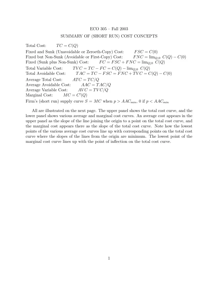
ECO 305 — Fall 2003 SUMMARY OF (SHORT RUN) COST CONCEPTS Total Cost: TC = C ( Q ) Fixed and Sunk (Unavoidable or Zeroeth-Copy) Cost: FSC = C (0) Fixed but Non-Sunk (Avoidable or First-Copy) Cost: FNC = lim Q ↓ 0 C ( Q ) − C (0) Fixed (Sunk plus Non-Sunk) Cost: FC = FSC + FNC = lim Q ↓ 0 C ( Q ) Total Variable Cost: TV C = TC − FC = C ( Q ) − lim Q ↓ 0 C ( Q ) Total Avoidable Cost: TAC = TC − FSC = FNC + TV C = C ( Q ) − C (0) Average Total Cost: ATC = TC/Q Average Avoidable Cost: AAC = TAC/Q Average Variable Cost: AV C = TV C/Q MC = C 0 ( Q ) Marginal Cost: Firm’s (short run) supply curve S = MC when p > AAC min , 0 if p < AAC min All are illustrated on the next page. The upper panel shows the total cost curve, and the lower panel shows various average and marginal cost curves. An average cost appears in the upper panel as the slope of the line joining the origin to a point on the total cost curve, and the marginal cost appears there as the slope of the total cost curve. Note how the lowest points of the various average cost curves line up with corresponding points on the total cost curve where the slopes of the lines from the origin are minimum. The lowest point of the marginal cost curve lines up with the point of in fl ection on the total cost curve. 1

. 2

EMPIRICAL EXAMPLES OF COST FUNCTIONS FUNCTIONS There is an extensive literature on the empirical estimation of production, pro fi t and cost functions. Discussions and surveys include Dale W. Jorgenson, Productivity, Vol. 2, MIT Press, 1995, and Ernst R. Berndt, The Practice of Econometrics, Addison-Wesley, 1991, Chapters 3, 9. In this course whose focus is theory, we can only o ff er a couple of examples. Berndt (pp. 469-476) estimates a cost function for U.S. manufacturing as a whole. This involves additional issues of aggregation over numerous fi rms, which we must skip over. Output Y is produced using capital K , labor L , energy E , and other intermediate inputs M . The cost C is assumed to have the form X X X α i ln( P i ) + 1 ln C = ln( α 0 ) + γ ij ln( P i ) ln( P j ) 2 i i j X 2 γ Y Y (ln Y ) 2 + + α Y ln Y + 1 γ iY ln( P i ) ln Y i where the various subscripted Greek letters are parameters, the P i are prices of the inputs, and the subscripts i and j run over the inputs K , L , E , and M . The following restrictions are imposed on the parameters (Why?): X X α i = 1 , γ ij = γ ji , γ ij = 0 for j = K , L , E , M , Y . i i Actually the estimation is done not on the cost function itself, but on the factor cost share functions that can be obtained from it using Hotelling’s (or Shepherd’s) Lemma; for example the share of wages in cost is P L L = P L ∂ C = d ln C . C C ∂ P L d ln P L The estimates of the coe ffi cients themselves are less interesting than their economic im- plications. Speci fi cally, from the input demand functions we can calculate the elasticities of substitution σ ij between any pair of inputs i and j . Berndt reports σ KL = 0 . 97 , σ KE = − 3 . 60 , σ KM = 0 . 35 , σ LM = 0 . 61 , σ EM = 0 . 83 , σ LE = 0 . 68 Thus all distinct pairs of inputs are substitutes (an increae in the price of one increases the demand for the other) except capital and energy which are quite strongly complements. If the cost function were Cobb-Douglas, all these cross-substitution elasticities would equal 1; most pairs show less substitution, except capital and labor which is almost at its Cobb-Douglas level. The own price elasticities of demands for the inputs are ² K = − 0 . 34 , ² L = − 0 . 45 , ² E = − 0 . 53 , ² M = − 0 . 24 . These again show substantially less substitution than Cobb-Douglas (in which case all the numbers would equal 1). 3

Unfortunately γ Y Y does not appear in the factor share equations (Why?), so Berndt does not estimate it and does not report whether his cost function shows increasing or decreasing returns to scale. But in Chapter 3 he surveys research on scale economies in U.S. electricity generation. The estimates show γ Y < 1 and γ Y Y > 0; thus the returns to scale are initially increasing for a range of small outputs but eventually decreasing for large scale (Why?). He also fi nds that the bulk of output was being produced “by fi rms operating in the essentially fl at area of the average cost curve.” Stephen Moeller, in his 1999 Princeton senior thesis, Cost Consequences of the Growth of U.S. Credit Unions: Information and Scale E ff ects, estimates a cost function for credit unions. His speci fi cation is of the Cobb-Douglas form: X X ln C = a + b 1 ln Q + b 2 (ln Q ) 2 + c i ln W i + d j ln F j + µ , i j where Q is a measure of the size (output) of the credit union, W i are factor prices, F j are other structural variables being controlled for, and µ is a stochastic error term. (Much thought and care is needed in choosing the appropriate measures of all these variables and then constructing the data sets; interested readers should consult the thesis for the details.) Here is a typical fi nding. Measuring the output by the total number of loans outstanding at the year’s end, Moeller fi nds the following coe ffi cient estimates for 1998: b 1 = 0 . 6537 with standard error 0.0231, b 2 = 0 . 0204 with standard error 0.0015. Thus both coe ffi cients are very tightly estimated. Since b 1 < 1, there are economies of scale, but since b 2 > 0, these eventually run out. The intuition is that a larger credit union gains the bene fi ts of better diversi fi cation and can spread its administrative overheads over a larger volume of business. But as it expands, it acquires a less coherent and more hetergeneous membership about which it has less information and over which it has less moral suasion; therefore it has a greater cost of default. Averge cost is minimized when ln Q = (1 − b 1 ) / (2 b 2 ) = 8 . 48 , or Q = 4764 . He fi nds that 85% of U.S. credit unions were actually to the left of this point. The median union had Q = 705. However, the average cost curve was pretty fl at near its bottom — comparing two unions that di ff er in size but are otherwise similar, the average cost of the median union was only 7.8 percent higher than that of the optimum-sized union. 4