Early Diagenesis Modelling with MEDUSA Guy Munhoven Laboratory for - PDF document

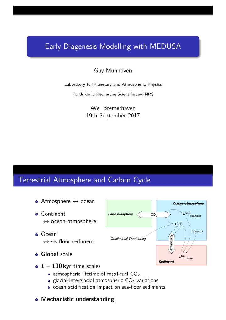
Early Diagenesis Modelling with MEDUSA Guy Munhoven Laboratory for Planetary and Atmospheric Physics Fonds de la Recherche Scientifique–FNRS AWI Bremerhaven 19th September 2017 Terrestrial Atmosphere and Carbon Cycle Atmosphere ↔ ocean Ocean−atmosphere Continent 13 Land biosphere δ C CO 2 seawater ↔ ocean-atmosphere 2− CO 3 species Ocean Carbonate Continental Weathering ↔ seafloor sediment Global scale 13 δ C foram Sediment 1 – 100 kyr time scales atmospheric lifetime of fossil-fuel CO 2 glacial-interglacial atmospheric CO 2 variations ocean acidification impact on sea-floor sediments Mechanistic understanding

Model Theory, Mathematical Methods and Development SOLVE_AT_GENERAL p H 5 12 Basic research 11 4 resolution methods 10 Alk T (meq/kg) 3 9 properties and limitations p H SWS 8 2 reliability 7 extension of existing methods 6 1 5 0 4 3 -1 Noteworthy outcomes 0 1 2 3 4 5 6 C T (mmol/kg) K¨ ohler et al. (Biogeosciences 2006) – Keeling plots Munhoven (Geoscientific Model Development 2013) – solving the pH-alkalinity equation (SolveSAPHE methods and library), adopted as the workhorse in MOCSY 2.0, to be used in the upcoming CMIP6 Ocean Model Intercomparison Project (OMIP) Acidification: Perturbation of the ocean-sediment exchange Marine carbonates: ocean-sediment exchange = [CO ] 3 = [CO ] in situ 3 CSH = [CO ] sat CCD 3 depth

Model Description MBM – Multi-Box Model of ocean-atmosphere carbon cycle ten oceanic and one atmospheric reservoirs realistic hypsometry fully coupled to . . . 304 copies of MEDUSA Model of Early Diagenesis in the Upper Sediment (A) bioturbated mixed-layer with 21 grid-points on top of a stack of thin layers (sediment core) solves time-dependent transport-reaction equations solids: calcite, aragonite, POM, clay 3 , CO 2 − solutes: CO 2 , HCO − 3 , O 2 fully bi-directional exchange between the two zones Full description: Munhoven, Deep-Sea Res. II (2007) Ocean Carbon Cycle Model MBM 90 ◦ N 50 ◦ N 40 ◦ S 40 ◦ S 40 ◦ N 65 ◦ N 0 m ✲ ✛ ✛ ✛ ✛ ✲ ❡ 1.7 3.7 0.3 1.3 0.8 ✛ ✲ ✛ ✲ ✛ ✲ ✛ ✲ a a ❡ SLATL SLI-P 0.3 0.1 1.9 0.3 ✻ ✻ 2.0 ❄ 1.0 ❄ 100 m 4.2 13.2 ❄ ❄ SNATL SANT SNPAC ✛ ✛ ✛ 1.8 ✲ 17.9 15.7 8.5 ✛ ✲ ✛ ✲ ✛ ✲ ✛ ✲ ILATL ILI-P 1.1 0.2 4.2 0.8 ✻ 5.2 ✻ ✻ ✻ 18.7 ✻ ✻ 0.3 ✻ ✻ 18.2 ❄ 6.0 ❄ 1000 m 1.0 2.8 8.1 3.2 0.2 ❄ ❄ ❄ ❄ ❄ 13.0 ✲ 19.0 ✲ ✛ ✲ ✛ ✲ DATL DANT DI-P 3.3 7.1 Fluxes in Sverdrup Atlantic Antarctic Indo-Pacific

Coupling MBM and MEDUSA MEDUSA Sediment Column Sedimentary mixed layer 21−node grid 10 cm 0 3 % CaCO 50 MBM Surface Reservoir 10 mm 100 Z 0 Z 1 Z 2 Historical Z MBM 3 Z 4 zone Intermediate Reservoir . . . Z j MBM Z j+1 Deep 100 m Reservoir . . . Z 79 Z 80 Sediment Model MEDUSA (Version 1) MEDUSA-v1 (Munhoven, 2007) Solids: clay, calcite, aragonite and organic matter 3 , CO 2 − Porewater solutes: CO 2 , HCO − and O 2 3 Unpublished #1 Solids: clay, calcite, aragonite, opal and organic matter 3 , CO 2 − Porewater solutes: CO 2 , HCO − 3 , O 2 and H 4 SiO 4 Unpublished #2 Solids: clay, calcite, aragonite, opal and organic matter; 13 C-calcite, 13 C-aragonite, 13 C-organic matter 3 , CO 2 − Porewater solutes: CO 2 , HCO − 3 , O 2 and H 4 SiO 4 ; 3 , 13 CO 2 − 13 CO 2 , H 13 CO − 3

Sediment Model MEDUSA (Version 1 to Version 2) Configurations assembled and selected by pre-processor directives Pre-processor directives cumbersome to use for complex code configuration Code became difficult to manage and extend with time Develop a scheme to have the code built from description files Similar to BRNS (Regnier et al., U. Utrecht, V. U. Brussels) or MEDIA (Meysman, NIOZ Yerseke) Sediment Model MEDUSA (Version 2) Flexible configuration composition: solid and solute components processes: includes extensible library of rate laws equilibria: includes extensible library of equilibrium relationships Configuration and descriptions based upon XML files extensible and flexible format uses Fortran 95 library µ XML to read XML files Code generator MEDUSACOCOGEN (also in Fortran 95)

Partitioning of the Model Sediment z=z W Diffusive Boundary Layer top DBL diffusion Solutes interconversion reactions z=z Sediment top T bioturbation advection Solids reactions diffusion REACLAY advection Solutes reactions z=z Z Bottom of bioturbation zone advection only Solids reactions diffusion advection Solutes reactions Bottom of modelled section z=z B z TRANLAY CORELAY preservation only Solids no reactions General Diagenesis Equation ∂ ˆ ∂ t + ∂ ˆ C i J i ∂ z − ˆ S i = 0 t is time z depth below the sediment-water interface ˆ C i is the concentration of i per unit volume of total sediment (solids plus porewater) in moles for solutes in kg for solids ˆ C i related to phase-specific concentrations C s i (for solids) and i (for solutes) by ˆ i and ˆ C f C i = (1 − ϕ ) C s C i = ϕ f C f i ˆ J i is the local transport (advection and diffusion), per unit surface area of total sediment

General Diagenesis Equation ∂ ˆ ∂ t + ∂ ˆ C i J i ∂ z − ˆ S i = 0 S i = ˆ ˆ r i + ˆ R i + ˆ Q i is the net source-minus-sink balance for constituent i , per unit volume of total sediment R i = ˆ ˆ P i − ˆ D i is the net reaction rate, i.e., the difference between ˆ P i ≥ 0, production rate ˆ D i ≥ 0, destruction or decay rate ˆ r i is the net fast reaction rate, filtered out by an equilibrium consideration ˆ Q i is the non-local transport (considered only for solutes). Transport Solids ∂ (1 − ϕ ) C s ∂ C s ˆ J i = − D inter − (1 − ϕ ) D intra ∂ z + (1 − ϕ ) wC s i i i i i ∂ z Solutes: local J i = − ϕ D sw ∂ C f ˆ i i ∂ z . θ 2 Solutes: non-local ˆ Q i ( z ) = α ( z ) ϕ f ( z )( C oc − C f i ( z )) i

Transport Common framework: evaluating transport terms compiling equation system and Jacobian solving the system (fully implicit in time, upwind biased in space) Application specific parts added by the Medusa Configuration and Code Generation tool MEDUSACOCOGEN Components (solids and solutes) Processes (chemical reactions) Chemical equilibria Solid Definition File: Calcite <? xml version ="1.0"?> 1 2 <Solid type="normal"> 3 4 <Names> 5 <Generic>Calcite</Generic> 6 <Long>Calcite</Long> 7 <ShortID>calc</ShortID> 8 </Names> 9 10 11 <PhysicalProperties> 12 <Density units="kg/m3">2700</Density> 13 <MolWeight units="kg/mol">0.1000869</MolWeight> 14 </PhysicalProperties> 15 16

Solid Definition File: Calcite 17 <ChemicalComposition> 18 <Ca>1</Ca> 19 <C> 1</C> 20 <O> 3</O> 21 </ChemicalComposition> 22 23 24 <CodeBits> 25 <SolubilityProduct units="molˆ2/mˆ6"> 26 <Fortran requireslibrary="libthdyct" 27 requires="wtmpk, wsalin, wdbsl, rho"> 28 <![ CDATA [ 29 {varname} = AKCALC(wtmpk, wsalin, wdbsl) * (rho**2) 30 ]]> 31 </Fortran> 32 </SolubilityProduct> 33 </CodeBits> 34 35 Solid Definition File: Calcite 36 <Alkalinity units="eq/mol">2</Alkalinity> 37 38 39 <ConservationProperties units="mol/mol"> 40 <C> 1</C> 41 </ConservationProperties> 42 43 </Solid> 44

Solute Definition File: CO 32 − <? xml version ="1.0"?> 1 2 <Solute type="normal"> 3 4 <Names> 5 <Generic>CO3</Generic> 6 <Long>Carbonate Ion</Long> 7 <ShortID>co3</ShortID> 8 </Names> 9 10 11 <ChemicalComposition> 12 <C> 1</C> 13 <O> 3</O> 14 </ChemicalComposition> 15 16 Solute Definition File: CO 32 − 17 <CodeBits> 18 <DiffCoeff> 19 <Fortran requires="wtmpdc"> 20 <![ CDATA [ 21 ! D_CO3 : from Boudreau (1997, Table 4.8, in cm2/s) 22 {varname} = 23 & (4.33D-6 + 0.199D-6*wtmpdc)*dp_cm2_p_sec 24 ]]> 25 </Fortran> 26 </DiffCoeff> 27 </CodeBits> 28 29 30 <Alkalinity units="eq/mol">2</Alkalinity> 31 32 33 <ConservationProperties units="mol/mol"> 34 <C> 1</C> 35 </ConservationProperties> 36 37 </Solute> 38