e / - Separation in AHCAL using shower shapes Justas Zalieckas AHCAL - - PowerPoint PPT Presentation

e
SMART_READER_LITE
LIVE PREVIEW

e / - Separation in AHCAL using shower shapes Justas Zalieckas AHCAL - - PowerPoint PPT Presentation

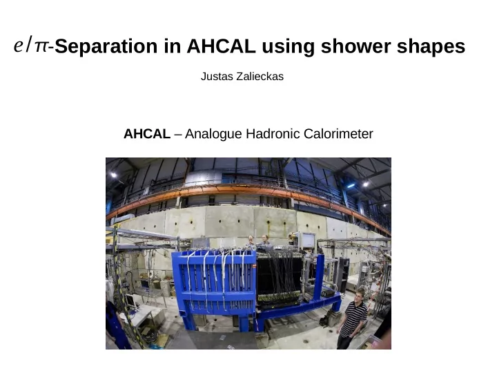
e / - Separation in AHCAL using shower shapes Justas Zalieckas AHCAL Analogue Hadronic Calorimeter Outline Analogue Hadronic Calorimeter (AHCAL) separation problem e / e / Shower shape variables for separation


slide-1
SLIDE 1

e/

  • Separation in AHCAL using shower shapes

Justas Zalieckas

AHCAL – Analogue Hadronic Calorimeter

slide-2
SLIDE 2

2

Outline

  • Analogue Hadronic Calorimeter (AHCAL)
  • separation problem
  • Shower shape variables for separation
  • Boosted Decision Trees (BDT) and Multivariate Data

Analysis (MDA)

  • Results
  • Conclusions

e/ e/

slide-3
SLIDE 3

3

Analogue Hadronic Calorimeter (AHCAL)

Used to determine the coordinates of the incident point of the particles on the calorimeter surface: xtrk and ytrk. Granularity: 3x3 cm2, 6x6 cm2, 12x12 cm2.

AHCAL

  • Sampling calorimeter
  • 30 layers of sandwich

structure

  • One layer – 10 mm W +

5 mm scintillator tiles

  • High scintillator

granularity

  • Wavelength shifting

fibers are read out with Silicon Photomultipliers (SiPM)

  • Cherenkov counters in

front of AHCAL

slide-4
SLIDE 4

4

separation problem

separation based on Cherenkov counters

  • efficiency for electron identification becomes low for low pressure
  • purity for electron identification drops with increasing pion content of the

beam

  • -> difficult to separate in low energy range (E<10 GeV)

Proposed solution

  • use shower shape information from calorimeter to distinguish between

electromagnetic and hadronic showers

  • combine information using multivariate data analysis technique

My tasks:

  • 1. Write Marlin processor to create ROOT files with trees containing

separation variables.

  • 2. Use TMVA 4 (Toolkit for Multivariate Data Analysis with ROOT) package with

created ROOT files for separation.

e/

e/ e/ e/

slide-5
SLIDE 5

5

  • Scatter plot of two shower

shape variables:

  • energy weighted radial distance
  • = energy of cell i
  • = energy sum in the first 5

AHCAL layers

  • = total energy sum
  • = cells center coordinates
  • Overlapping regions
  • 5 GeV samples
  • For better electrons

separation – use more shower shape variables

separation problem

d=∑ Eixi−xtrk

2 yi− ytrk 2

∑ Ei

E5 Etot

e/

Ei xi, yi

slide-6
SLIDE 6

6

Shower shape variables for separation

  • energy weighted radial

distance

  • = fraction of

contained in the first 5 layers

  • third momentum of

radial distance

  • energy density
  • = cell volume
  • = cells number

E5/Etot d1[mm] logd 3[mm]

d1=∑ Eixi−xtrk2 yi−ytrk2

∑ Ei

e/

Energy density[MIPs/cm

3]

∑ Ei/V i

N

d3=∑ Ei

3xi−xtrk2 yi−ytrk2

∑ Ei

3

E5/Etot Etot

V i N

slide-7
SLIDE 7

7

Shower shape variables for separation

  • second momentum
  • f radial distance
  • radial distance

containing 90%

  • number of hits

containing 90%

  • total hits number
  • is fraction of

cells containing 90%

  • f
  • cells average energy

e/

Etot Etot

R90[mm]

R90

N 90/N

N 90 N

∑ Ei

N

Cellsaverage energy[MIPs] d 2[mm]

d2=∑ Ei

3xi−xtrk2 yi− ytrk2

∑ Ei

2

N 90/N

Etot

slide-8
SLIDE 8

8

Shower shape variables for separation

  • maximum energy

loss layer number

  • shower start layer

number

  • is number of

layers to reach shower maximum

e/

Max.energylosslayernumber Lmax Shower start layer number Lstart Lmax−Lstart

Lmax Lstart Lmax−Lstart

slide-9
SLIDE 9

9

Decision tree for events classification

  • Leaf node
  • Root node
  • Events sample
  • Classification/separation

variables for split decisions

  • Repeated yes/no split decisions
  • Phase space is divided in many

regions

  • Events end in final leaf node
  • Purity

WS, WB – signal and background weights. If p>0.5 – signal, if p<0.5 - background. p=

S

W S

S

W S∑

B

W B

slide-10
SLIDE 10

10

Boosted Decision Trees

Boosting the decision tree

  • Reweight events
  • New trees are derived from the

same training sample

  • Trees form a forest
  • Average weights

(misclassification)

  • Combine into a single classifier
  • Test classifier with test sample
  • Boosting stabilizes fluctuations

in the training sample and considerably enhances classifier performance w.r.t. a single tree.

W iW ie

f err

W i Training sample Single classifier Testing sample

slide-11
SLIDE 11

11

Correlation of input variables for signal

Correlation matrix for electrons

slide-12
SLIDE 12

12

Correlation of input variables for background

Correlation matrix for pions

slide-13
SLIDE 13

13

Results

  • Variable ranking:

Rank Variable Importance 1 N90/N 1.288e-01 2 d1 1.269e-01 3 E5/Etot 1.165e-01 4 d2 1.145e-01 5

Energy density

1.100e-01 6 R90 1.018e-01 7 d3 1.015e-01 8 Lstart 7.623e-02 9

Cells average energy

6.687e-02 10 Lmax 4.406e-02

11 Lmax-Lstart

1.272e-02

Electron: 22586 (training), 22587 (testing). Pion: 18045 (training), 18046 (testing).

slide-14
SLIDE 14

14

Results

Input variables in BDT Electron eff. with contamination fraction effpion=0.01 Electron eff. with contamination fraction effpion=0.1 Separation <S2> d1, E5/Etot

0.977 1 0.956

N90/N, d1, E5/Etot, d2, Energy density, R90, d3

0.988 1 0.97

N90/N, d1, E5/Etot, d2, Energy density, R90, d3, Lstart, Cells average energy, Lmax, Lmax-Lstart

0.991 1 0.973

Input variables in

  • ptimized Cut

method d1, E5/Etot

0.975 0.992

  • eff pion= N pion. selected

N pion.total 〈S

2〉=1

2

∫ yel.−y pion2

yel.y pion dy

  • Electron efficiency
  • Pion efficiency
  • Separation

is PDFs of classifier .

is 1 with no overlap and is 0 with full overlap. eff el.=N el.selected Nel.total yel., y pion y 〈S

2〉

Cut on and gives . Using BDT with 11 input variables for:

  • -->
  • -->
  • -> Large improvement with

multivariate selection.

E5/Etot≥0.875 d1≤40 eff el.=0.48,eff pion=0.00047 eff el.=0.48 eff pion=0.00047 eff pion=0.00027 eff el.=0.61

slide-15
SLIDE 15

15

Conclusions

  • Increase in input variables number increases electron

separation efficiency

  • BDT classifier allows better electron/pion separation

than simple cut method

  • Further analysis with real data sample