[PPT] - E-M method for latent variable models Define augmented likelihood n PowerPoint Presentation

SLIDE 1

E-M method for latent variable models

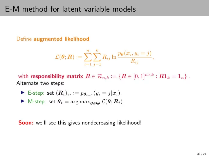
Define augmented likelihood L(θ; R) :=

n

i=1

k

j=1

Rij ln pθ(xi, yi = j) Rij , with responsibility matrix R ∈ Rn,k := {R ∈ [0, 1]n×k : R1k = 1n} . Alternate two steps: ◮ E-step: set (Rt)ij := pθt−1(yi = j|xi). ◮ M-step: set θt = arg maxθ∈Θ L(θ; Rt). Soon: we’ll see this gives nondecreasing likelihood!

30 / 70

SLIDE 2

E-M for Gaussian mixtures

Initialization: a standard choice is πj = 1/k, Σj = I, and (µj)k

j=1 given

by k-means. ◮ E-step: Set Rij = pθ(yi = j|xi), meaning Rij = pθ(yi = j|xi) = pθ(yi = j, xi) pθ(xi) = πjpµj,Σj(xi) k

l=1 πlpµl,Σl(xi)

. ◮ M-step: solve arg maxθ∈Θ L(θ; R), meaning πj := n

i=1 Rij

n

i=1

k

l=1 Ril

= n

i=1 Rij

n , µj := n

i=1 Rijxi

n

i=1 Rij

= n

i=1 Rijxi

nπj , Σj := n

i=1 Rij(xi − µj)(xi − µj)T

nπj . (These are as before.)

31 / 70

SLIDE 3

Demo: spherical clusters

2 2 4 6 8 10 2 2 4 6

(Initialized with k-means, thus not so dramatic.)

32 / 70

SLIDE 4

Demo: spherical clusters

2 2 4 6 8 10 2 2 4 6

(Initialized with k-means, thus not so dramatic.)

32 / 70

SLIDE 5

Demo: spherical clusters

2 2 4 6 8 10 2 2 4 6

(Initialized with k-means, thus not so dramatic.)

32 / 70

SLIDE 6

Demo: spherical clusters

2 2 4 6 8 10 2 2 4 6

(Initialized with k-means, thus not so dramatic.)

32 / 70

SLIDE 7

Demo: spherical clusters

2 2 4 6 8 10 2 2 4 6

(Initialized with k-means, thus not so dramatic.)

32 / 70

SLIDE 8

Demo: spherical clusters

2 2 4 6 8 10 2 2 4 6

(Initialized with k-means, thus not so dramatic.)

32 / 70

SLIDE 9

Demo: spherical clusters

2 2 4 6 8 10 2 2 4 6

(Initialized with k-means, thus not so dramatic.)

32 / 70

SLIDE 10

Demo: spherical clusters

2 2 4 6 8 10 2 2 4 6

(Initialized with k-means, thus not so dramatic.)

32 / 70

SLIDE 11

Demo: spherical clusters

2 2 4 6 8 10 2 2 4 6

(Initialized with k-means, thus not so dramatic.)

32 / 70

SLIDE 12

Demo: spherical clusters

2 2 4 6 8 10 2 2 4 6

(Initialized with k-means, thus not so dramatic.)

32 / 70

SLIDE 13

Demo: elliptical clusters

E. . .

5 5 10 15 10.0 7.5 5.0 2.5 0.0 2.5 5.0 7.5 10.0 33 / 70

SLIDE 14

Demo: elliptical clusters

E. . . M. . .

5 5 10 15 10.0 7.5 5.0 2.5 0.0 2.5 5.0 7.5 10.0 33 / 70

SLIDE 15

Demo: elliptical clusters

E. . . M. . . E. . .

5 5 10 15 10.0 7.5 5.0 2.5 0.0 2.5 5.0 7.5 10.0 33 / 70

SLIDE 16

Demo: elliptical clusters

E. . . M. . . E. . . M. . .

5 5 10 15 10.0 7.5 5.0 2.5 0.0 2.5 5.0 7.5 10.0 33 / 70

SLIDE 17

Demo: elliptical clusters

E. . . M. . . E. . . M. . . E. . .

5 5 10 15 10.0 7.5 5.0 2.5 0.0 2.5 5.0 7.5 10.0 33 / 70

SLIDE 18

Demo: elliptical clusters

E. . . M. . . E. . . M. . . E. . . M. . .

5 5 10 15 10.0 7.5 5.0 2.5 0.0 2.5 5.0 7.5 10.0 33 / 70

SLIDE 19

Demo: elliptical clusters

E. . . M. . . E. . . M. . . E. . . M. . . E. . .

5 5 10 15 10.0 7.5 5.0 2.5 0.0 2.5 5.0 7.5 10.0 33 / 70

SLIDE 20

Demo: elliptical clusters

E. . . M. . . E. . . M. . . E. . . M. . . E. . . M. . .

5 5 10 15 10.0 7.5 5.0 2.5 0.0 2.5 5.0 7.5 10.0 33 / 70

SLIDE 21

Demo: elliptical clusters

E. . . M. . . E. . . M. . . E. . . M. . . E. . . M. . .

5 5 10 15 10.0 7.5 5.0 2.5 0.0 2.5 5.0 7.5 10.0 33 / 70

SLIDE 22

Demo: elliptical clusters

E. . . M. . . E. . . M. . . E. . . M. . . E. . . M. . .

5 5 10 15 10.0 7.5 5.0 2.5 0.0 2.5 5.0 7.5 10.0 33 / 70

SLIDE 23

Demo: elliptical clusters

E. . . M. . . E. . . M. . . E. . . M. . . E. . . M. . .

10 5 5 10 15 10.0 7.5 5.0 2.5 0.0 2.5 5.0 7.5 33 / 70

SLIDE 24

Demo: elliptical clusters

E. . . M. . . E. . . M. . . E. . . M. . . E. . . M. . .

10 5 5 10 15 10.0 7.5 5.0 2.5 0.0 2.5 5.0 7.5 33 / 70

SLIDE 25

Demo: elliptical clusters

E. . . M. . . E. . . M. . . E. . . M. . . E. . . M. . .

10 5 5 10 15 10.0 7.5 5.0 2.5 0.0 2.5 5.0 7.5 33 / 70

SLIDE 26

Demo: elliptical clusters

E. . . M. . . E. . . M. . . E. . . M. . . E. . . M. . .

10 5 5 10 15 10.0 7.5 5.0 2.5 0.0 2.5 5.0 7.5 33 / 70

SLIDE 27

Demo: elliptical clusters

E. . . M. . . E. . . M. . . E. . . M. . . E. . . M. . .

10 5 5 10 15 10.0 7.5 5.0 2.5 0.0 2.5 5.0 7.5 33 / 70

SLIDE 28

Demo: elliptical clusters

E. . . M. . . E. . . M. . . E. . . M. . . E. . . M. . .

10 5 5 10 15 10.0 7.5 5.0 2.5 0.0 2.5 5.0 7.5 33 / 70

SLIDE 29

Demo: elliptical clusters

E. . . M. . . E. . . M. . . E. . . M. . . E. . . M. . .

10 5 5 10 15 10.0 7.5 5.0 2.5 0.0 2.5 5.0 7.5 33 / 70

SLIDE 30

Demo: elliptical clusters

E. . . M. . . E. . . M. . . E. . . M. . . E. . . M. . .

10 5 5 10 15 10.0 7.5 5.0 2.5 0.0 2.5 5.0 7.5 33 / 70

SLIDE 31

Demo: elliptical clusters

E. . . M. . . E. . . M. . . E. . . M. . . E. . . M. . .

10 5 5 10 15 10.0 7.5 5.0 2.5 0.0 2.5 5.0 7.5 33 / 70

SLIDE 32

Demo: elliptical clusters

E. . . M. . . E. . . M. . . E. . . M. . . E. . . M. . .

10 5 5 10 15 10.0 7.5 5.0 2.5 0.0 2.5 5.0 7.5 33 / 70

SLIDE 33

Demo: elliptical clusters

E. . . M. . . E. . . M. . . E. . . M. . . E. . . M. . .

10 5 5 10 15 10.0 7.5 5.0 2.5 0.0 2.5 5.0 7.5 33 / 70

SLIDE 34

Demo: elliptical clusters

E. . . M. . . E. . . M. . . E. . . M. . . E. . . M. . .

10 5 5 10 15 10.0 7.5 5.0 2.5 0.0 2.5 5.0 7.5 33 / 70

SLIDE 35

Demo: elliptical clusters

E. . . M. . . E. . . M. . . E. . . M. . . E. . . M. . .

10 5 5 10 15 10.0 7.5 5.0 2.5 0.0 2.5 5.0 7.5 33 / 70

SLIDE 36

Demo: elliptical clusters

E. . . M. . . E. . . M. . . E. . . M. . . E. . . M. . .

10 5 5 10 15 10.0 7.5 5.0 2.5 0.0 2.5 5.0 7.5 33 / 70

SLIDE 37

Demo: elliptical clusters

E. . . M. . . E. . . M. . . E. . . M. . . E. . . M. . .

10 5 5 10 15 10.0 7.5 5.0 2.5 0.0 2.5 5.0 7.5 33 / 70

SLIDE 38

Demo: elliptical clusters

E. . . M. . . E. . . M. . . E. . . M. . . E. . . M. . .

10 5 5 10 15 10.0 7.5 5.0 2.5 0.0 2.5 5.0 7.5 33 / 70

SLIDE 39

Demo: elliptical clusters

E. . . M. . . E. . . M. . . E. . . M. . . E. . . M. . .

10 5 5 10 15 10.0 7.5 5.0 2.5 0.0 2.5 5.0 7.5 33 / 70

SLIDE 40

Demo: elliptical clusters

E. . . M. . . E. . . M. . . E. . . M. . . E. . . M. . .

10 5 5 10 15 10.0 7.5 5.0 2.5 0.0 2.5 5.0 7.5 33 / 70

SLIDE 41

Theorem. Suppose (R0, θ0) ∈ Rn,k × Θ arbitrary, thereafter (Rt, θt) given by E-M: (Rt)ij := pθt−1(y = j|xi). and θt := arg max

θ∈Θ

L(θ; Rt) Then L(θt; Rt) ≤ max

R∈Rn×k L(θt; R) = L(θt; Rt+1) = L(θt)

≤ L(θt+1; Rt+1). In particular, L(θt) ≤ L(θt+1).

34 / 70

SLIDE 42

Theorem. Suppose (R0, θ0) ∈ Rn,k × Θ arbitrary, thereafter (Rt, θt) given by E-M: (Rt)ij := pθt−1(y = j|xi). and θt := arg max

θ∈Θ

L(θ; Rt) Then L(θt; Rt) ≤ max

R∈Rn×k L(θt; R) = L(θt; Rt+1) = L(θt)

≤ L(θt+1; Rt+1). In particular, L(θt) ≤ L(θt+1). Remarks. ◮ We proved a similar guarantee for k-means, which is also an alternating minimization scheme. ◮ Similarly, MLE for Gaussian mixtures is NP-hard; it is also known to need exponentially many samples in k to information-theoretically recover the parameters.

34 / 70

SLIDE 43

Proof. We’ve already shown:

◮ L(θt; Rt+1) = L(θt); ◮ L(θt; Rt+1) = maxθ∈Θ L(θ; Rt+1) ≤ L(θt+1; Rt+1) by definition

f θt+1.

We still need to show: L(θt; Rt+1) = maxR∈Rn,k L(θt+1; R). We’ll give two proofs.

35 / 70

SLIDE 44

Proof. We’ve already shown:

◮ L(θt; Rt+1) = L(θt); ◮ L(θt; Rt+1) = maxθ∈Θ L(θ; Rt+1) ≤ L(θt+1; Rt+1) by definition

f θt+1.

We still need to show: L(θt; Rt+1) = maxR∈Rn,k L(θt+1; R). We’ll give two proofs. By concavity of ln (“Jensen’s inequality” in convexity lectures), for any R ∈ Rn,k, L(θt; R) =

n

i=1

k

j=1

Rij ln pθt(xi, yi = j) Rij ≤

n

i=1

ln  

k

j=1

Rij pθt(xi, yi = j) Rij   =

n

i=1

ln pθt(xi) = L(θt) = L(θt; Rt+1). Since R was arbitrary, maxR∈R L(θt; R) = L(θt; Rt+1).

35 / 70

SLIDE 45

Proof (continued). Here’s a second proof of that missing fact. To evaluate arg maxR∈Rn,k L(θ; R), consider Lagrangian

n

i=1

 

k

j=1

Rij ln pθ(xi, y = j) −

k

j=1

Rij ln Rij + λi k

j=1

Rij − 1



 . Fixing i and taking the gradient with respect to Rij for any j, 0 = ln pθ(xi, yi = j) − ln Rij − 1 + λi, giving Rij = pθ(xi, y = j) exp(λi − 1). Since moreover 1 =

j

Rij = exp(λi − 1)

j

pθ(xi, y = j) = exp(λi − 1)pθ(xi), it follows that exp(λi − 1) = 1/pθ(xi), and the optimal R satisfies Rij = pθ(xi,y=j)/pθ(xi) = pθ(y = j|xi).

36 / 70

SLIDE 46

Related issues.

37 / 70

SLIDE 47

Parameter constraints.

E-M for GMMs still works if we freeze or constrain some parameters.

38 / 70

SLIDE 48

Parameter constraints.

E-M for GMMs still works if we freeze or constrain some parameters. Examples: ◮ No weights: initialize π = (1/k, . . . , 1/k) and never update it. ◮ Diagonal covariance matrices: update everything as before, except Σj := diag((σj)2

1, . . . , (σj)2 d) where

(σj)2

l :=

n

i=1 Rij(xi − µj)2 l

nπj ; that is: we use coordinate-wise sample variances weighted by R. Why is this a good idea?

38 / 70

SLIDE 49

Parameter constraints.

E-M for GMMs still works if we freeze or constrain some parameters. Examples: ◮ No weights: initialize π = (1/k, . . . , 1/k) and never update it. ◮ Diagonal covariance matrices: update everything as before, except Σj := diag((σj)2

1, . . . , (σj)2 d) where

(σj)2

l :=

n

i=1 Rij(xi − µj)2 l

nπj ; that is: we use coordinate-wise sample variances weighted by R. Why is this a good idea? Computation (of inverse), sample complexity, . . .

38 / 70

SLIDE 50

Gaussian Mixture Model with diagonal covariances.

5 5 10 15 10.0 7.5 5.0 2.5 0.0 2.5 5.0 7.5 10.0 39 / 70

SLIDE 51

Gaussian Mixture Model with diagonal covariances.

5 5 10 15 10.0 7.5 5.0 2.5 0.0 2.5 5.0 7.5 10.0 39 / 70

SLIDE 52

Gaussian Mixture Model with diagonal covariances.

5 5 10 15 10.0 7.5 5.0 2.5 0.0 2.5 5.0 7.5 10.0 39 / 70

SLIDE 53

Gaussian Mixture Model with diagonal covariances.

5 5 10 15 10.0 7.5 5.0 2.5 0.0 2.5 5.0 7.5 10.0 39 / 70

SLIDE 54

Gaussian Mixture Model with diagonal covariances.

5 5 10 15 10.0 7.5 5.0 2.5 0.0 2.5 5.0 7.5 10.0 39 / 70

SLIDE 55

Gaussian Mixture Model with diagonal covariances.

5 5 10 15 10.0 7.5 5.0 2.5 0.0 2.5 5.0 7.5 10.0 39 / 70

SLIDE 56

Gaussian Mixture Model with diagonal covariances.

5 5 10 15 10.0 7.5 5.0 2.5 0.0 2.5 5.0 7.5 10.0 39 / 70

SLIDE 57

Gaussian Mixture Model with diagonal covariances.

5 5 10 15 10.0 7.5 5.0 2.5 0.0 2.5 5.0 7.5 10.0 39 / 70

SLIDE 58

Gaussian Mixture Model with diagonal covariances.

5 5 10 15 10.0 7.5 5.0 2.5 0.0 2.5 5.0 7.5 10.0 39 / 70

SLIDE 59

Gaussian Mixture Model with diagonal covariances.

5 5 10 15 10.0 7.5 5.0 2.5 0.0 2.5 5.0 7.5 10.0 39 / 70

SLIDE 60

Gaussian Mixture Model with diagonal covariances.

5 5 10 15 10.0 7.5 5.0 2.5 0.0 2.5 5.0 7.5 10.0 39 / 70

SLIDE 61

Gaussian Mixture Model with diagonal covariances.

5 5 10 15 10.0 7.5 5.0 2.5 0.0 2.5 5.0 7.5 10.0 39 / 70

SLIDE 62

Gaussian Mixture Model with diagonal covariances.

10 5 5 10 15 10.0 7.5 5.0 2.5 0.0 2.5 5.0 7.5 39 / 70

SLIDE 63

Gaussian Mixture Model with diagonal covariances.

10 5 5 10 15 10.0 7.5 5.0 2.5 0.0 2.5 5.0 7.5 39 / 70

SLIDE 64

Gaussian Mixture Model with diagonal covariances.

10 5 5 10 15 10.0 7.5 5.0 2.5 0.0 2.5 5.0 7.5 39 / 70

SLIDE 65

Gaussian Mixture Model with diagonal covariances.

10 5 5 10 15 10.0 7.5 5.0 2.5 0.0 2.5 5.0 7.5 39 / 70

SLIDE 66

Gaussian Mixture Model with diagonal covariances.

10 5 5 10 15 10.0 7.5 5.0 2.5 0.0 2.5 5.0 7.5 39 / 70

SLIDE 67

Gaussian Mixture Model with diagonal covariances.

10 5 5 10 15 10.0 7.5 5.0 2.5 0.0 2.5 5.0 7.5 39 / 70

SLIDE 68

Gaussian Mixture Model with diagonal covariances.

10 5 5 10 15 10.0 7.5 5.0 2.5 0.0 2.5 5.0 7.5 39 / 70

SLIDE 69

Gaussian Mixture Model with diagonal covariances.

10 5 5 10 15 10.0 7.5 5.0 2.5 0.0 2.5 5.0 7.5 39 / 70

SLIDE 70

Gaussian Mixture Model with diagonal covariances.

10 5 5 10 15 10.0 7.5 5.0 2.5 0.0 2.5 5.0 7.5 39 / 70

SLIDE 71

Gaussian Mixture Model with diagonal covariances.

10 5 5 10 15 10.0 7.5 5.0 2.5 0.0 2.5 5.0 7.5 39 / 70

SLIDE 72

Gaussian Mixture Model with diagonal covariances.

10 5 5 10 15 10.0 7.5 5.0 2.5 0.0 2.5 5.0 7.5 39 / 70

SLIDE 73

Gaussian Mixture Model with diagonal covariances.

10 5 5 10 15 10.0 7.5 5.0 2.5 0.0 2.5 5.0 7.5 39 / 70

SLIDE 74

Gaussian Mixture Model with diagonal covariances.

10 5 5 10 15 10.0 7.5 5.0 2.5 0.0 2.5 5.0 7.5 39 / 70

SLIDE 75

Gaussian Mixture Model with diagonal covariances.

10 5 5 10 15 10.0 7.5 5.0 2.5 0.0 2.5 5.0 7.5 39 / 70

SLIDE 76

Gaussian Mixture Model with diagonal covariances.

10 5 5 10 15 10.0 7.5 5.0 2.5 0.0 2.5 5.0 7.5 39 / 70

SLIDE 77

Gaussian Mixture Model with diagonal covariances.

10 5 5 10 15 10.0 7.5 5.0 2.5 0.0 2.5 5.0 7.5 39 / 70

SLIDE 78

Gaussian Mixture Model with diagonal covariances.

10 5 5 10 15 10.0 7.5 5.0 2.5 0.0 2.5 5.0 7.5 39 / 70

SLIDE 79

Gaussian Mixture Model with diagonal covariances.

10 5 5 10 15 10.0 7.5 5.0 2.5 0.0 2.5 5.0 7.5 39 / 70

SLIDE 80

Gaussian Mixture Model with diagonal covariances.

10 5 5 10 15 10.0 7.5 5.0 2.5 0.0 2.5 5.0 7.5 39 / 70

SLIDE 81

Gaussian Mixture Model with diagonal covariances.

10 5 5 10 15 10.0 7.5 5.0 2.5 0.0 2.5 5.0 7.5 39 / 70

SLIDE 82

Singularities

E-M with GMMs suffers from singularities: trivial situations where the likelihood goes to ∞ but the solution is bad. ◮ Suppose: d = 1, k = 2, πj = 1/2, n = 3 with x1 = −1 and x2 = +1 and x3 = +3. Initialize with µ1 = 0 and σ1 = 1, but µ2 = +3 = x3 and σ2 = 1/100. Then σ2 → 0 and L ↑ ∞.

40 / 70

SLIDE 83

Interpolating between k-means and GMM E-M

Same M-step: fix π = (1/k, . . . , 1/k) and Σj = cI for a fixed c > 0.

41 / 70

SLIDE 84

Interpolating between k-means and GMM E-M

Same M-step: fix π = (1/k, . . . , 1/k) and Σj = cI for a fixed c > 0. Same E-step: define qij := 1

2xi − µj2; the E-step chooses

Rij := pθ(yi = j|xi) = pθ(yi = j, xi) pθ(xi) = pθ(yi = j, xi) k

l=1 pθ(yi = l, xi)

= πjpµj,Σj(xi) k

l=1 πlpµl,Σl(xi)

= exp(−qij/c) k

l=1 exp(−qil/c)

Fix i ∈ {1, . . . , n} and suppose minimum qi := minj qij is unique:

41 / 70

SLIDE 85

Interpolating between k-means and GMM E-M

Same M-step: fix π = (1/k, . . . , 1/k) and Σj = cI for a fixed c > 0. Same E-step: define qij := 1

2xi − µj2; the E-step chooses

Rij := pθ(yi = j|xi) = pθ(yi = j, xi) pθ(xi) = pθ(yi = j, xi) k

l=1 pθ(yi = l, xi)

= πjpµj,Σj(xi) k

l=1 πlpµl,Σl(xi)

= exp(−qij/c) k

l=1 exp(−qil/c)

Fix i ∈ {1, . . . , n} and suppose minimum qi := minj qij is unique: lim

c↓0 Rij = lim c↓0

exp(−qij/c) k

l=1 exp(−qil/c)

= lim

c↓0

exp(qi − qij/c) k

l=1 exp(qi − qil/c)

=

1

qij = qi, qij = qi. That is, R becomes hard assignment A as c ↓ 0.

41 / 70

SLIDE 86

Interpolating between k-means and GMM E-M (part 2)

We can interpolate algorithmically, meaning we can create algorithms that have elements of both. Here’s something like k-means but with weights and covariances.

5 5 10 15 10.0 7.5 5.0 2.5 0.0 2.5 5.0 7.5 10.0 42 / 70

SLIDE 87

Interpolating between k-means and GMM E-M (part 2)

We can interpolate algorithmically, meaning we can create algorithms that have elements of both. Here’s something like k-means but with weights and covariances.

5 5 10 15 10.0 7.5 5.0 2.5 0.0 2.5 5.0 7.5 10.0 42 / 70

SLIDE 88

Interpolating between k-means and GMM E-M (part 2)

We can interpolate algorithmically, meaning we can create algorithms that have elements of both. Here’s something like k-means but with weights and covariances.

5 5 10 15 10.0 7.5 5.0 2.5 0.0 2.5 5.0 7.5 10.0 42 / 70

SLIDE 89

Interpolating between k-means and GMM E-M (part 2)

We can interpolate algorithmically, meaning we can create algorithms that have elements of both. Here’s something like k-means but with weights and covariances.

5 5 10 15 10.0 7.5 5.0 2.5 0.0 2.5 5.0 7.5 10.0 42 / 70

SLIDE 90

Interpolating between k-means and GMM E-M (part 2)

We can interpolate algorithmically, meaning we can create algorithms that have elements of both. Here’s something like k-means but with weights and covariances.

5 5 10 15 10.0 7.5 5.0 2.5 0.0 2.5 5.0 7.5 10.0 42 / 70

SLIDE 91

Interpolating between k-means and GMM E-M (part 2)

We can interpolate algorithmically, meaning we can create algorithms that have elements of both. Here’s something like k-means but with weights and covariances.

5 5 10 15 10.0 7.5 5.0 2.5 0.0 2.5 5.0 7.5 10.0 42 / 70

SLIDE 92

Interpolating between k-means and GMM E-M (part 2)

We can interpolate algorithmically, meaning we can create algorithms that have elements of both. Here’s something like k-means but with weights and covariances.

5 5 10 15 10.0 7.5 5.0 2.5 0.0 2.5 5.0 7.5 10.0 42 / 70

SLIDE 93

Interpolating between k-means and GMM E-M (part 2)

We can interpolate algorithmically, meaning we can create algorithms that have elements of both. Here’s something like k-means but with weights and covariances.

5 5 10 15 10.0 7.5 5.0 2.5 0.0 2.5 5.0 7.5 10.0 42 / 70

SLIDE 94

Interpolating between k-means and GMM E-M (part 2)

We can interpolate algorithmically, meaning we can create algorithms that have elements of both. Here’s something like k-means but with weights and covariances.

5 5 10 15 10.0 7.5 5.0 2.5 0.0 2.5 5.0 7.5 10.0 42 / 70

SLIDE 95

Interpolating between k-means and GMM E-M (part 2)

We can interpolate algorithmically, meaning we can create algorithms that have elements of both. Here’s something like k-means but with weights and covariances.

5 5 10 15 10.0 7.5 5.0 2.5 0.0 2.5 5.0 7.5 10.0 42 / 70

SLIDE 96

Interpolating between k-means and GMM E-M (part 2)

We can interpolate algorithmically, meaning we can create algorithms that have elements of both. Here’s something like k-means but with weights and covariances.

5 5 10 15 10.0 7.5 5.0 2.5 0.0 2.5 5.0 7.5 10.0 42 / 70

SLIDE 97

Interpolating between k-means and GMM E-M (part 2)

We can interpolate algorithmically, meaning we can create algorithms that have elements of both. Here’s something like k-means but with weights and covariances.

5 5 10 15 10.0 7.5 5.0 2.5 0.0 2.5 5.0 7.5 10.0 42 / 70

SLIDE 98

Interpolating between k-means and GMM E-M (part 2)

We can interpolate algorithmically, meaning we can create algorithms that have elements of both. Here’s something like k-means but with weights and covariances.

10 5 5 10 15 10.0 7.5 5.0 2.5 0.0 2.5 5.0 7.5 42 / 70

SLIDE 99

Interpolating between k-means and GMM E-M (part 2)

We can interpolate algorithmically, meaning we can create algorithms that have elements of both. Here’s something like k-means but with weights and covariances.

10 5 5 10 15 10.0 7.5 5.0 2.5 0.0 2.5 5.0 7.5 42 / 70

SLIDE 100

Interpolating between k-means and GMM E-M (part 2)

We can interpolate algorithmically, meaning we can create algorithms that have elements of both. Here’s something like k-means but with weights and covariances.

10 5 5 10 15 10.0 7.5 5.0 2.5 0.0 2.5 5.0 7.5 42 / 70

SLIDE 101

Interpolating between k-means and GMM E-M (part 2)

We can interpolate algorithmically, meaning we can create algorithms that have elements of both. Here’s something like k-means but with weights and covariances.

10 5 5 10 15 10.0 7.5 5.0 2.5 0.0 2.5 5.0 7.5 42 / 70

SLIDE 102

Interpolating between k-means and GMM E-M (part 2)

We can interpolate algorithmically, meaning we can create algorithms that have elements of both. Here’s something like k-means but with weights and covariances.

10 5 5 10 15 10.0 7.5 5.0 2.5 0.0 2.5 5.0 7.5 42 / 70

SLIDE 103

Interpolating between k-means and GMM E-M (part 2)

We can interpolate algorithmically, meaning we can create algorithms that have elements of both. Here’s something like k-means but with weights and covariances.

10 5 5 10 15 10.0 7.5 5.0 2.5 0.0 2.5 5.0 7.5 42 / 70

SLIDE 104

Interpolating between k-means and GMM E-M (part 2)

We can interpolate algorithmically, meaning we can create algorithms that have elements of both. Here’s something like k-means but with weights and covariances.

10 5 5 10 15 10.0 7.5 5.0 2.5 0.0 2.5 5.0 7.5 42 / 70

SLIDE 105

Interpolating between k-means and GMM E-M (part 2)

We can interpolate algorithmically, meaning we can create algorithms that have elements of both. Here’s something like k-means but with weights and covariances.

10 5 5 10 15 10.0 7.5 5.0 2.5 0.0 2.5 5.0 7.5 42 / 70

SLIDE 106

Interpolating between k-means and GMM E-M (part 2)

We can interpolate algorithmically, meaning we can create algorithms that have elements of both. Here’s something like k-means but with weights and covariances.

10 5 5 10 15 10.0 7.5 5.0 2.5 0.0 2.5 5.0 7.5 42 / 70

SLIDE 107

Interpolating between k-means and GMM E-M (part 2)

We can interpolate algorithmically, meaning we can create algorithms that have elements of both. Here’s something like k-means but with weights and covariances.

10 5 5 10 15 10.0 7.5 5.0 2.5 0.0 2.5 5.0 7.5 42 / 70

SLIDE 108

Interpolating between k-means and GMM E-M (part 2)

We can interpolate algorithmically, meaning we can create algorithms that have elements of both. Here’s something like k-means but with weights and covariances.

10 5 5 10 15 10.0 7.5 5.0 2.5 0.0 2.5 5.0 7.5 42 / 70

SLIDE 109

Interpolating between k-means and GMM E-M (part 2)

We can interpolate algorithmically, meaning we can create algorithms that have elements of both. Here’s something like k-means but with weights and covariances.

10 5 5 10 15 10.0 7.5 5.0 2.5 0.0 2.5 5.0 7.5 42 / 70

SLIDE 110

Summary of MLE part 2

43 / 70

SLIDE 111

Summary of MLE part 2

◮ Generative definition (“sampling story”)

f Gaussian mixture models (GMMs).

◮ PDF of GMMs. ◮ E-M in general, and what it guarantees. ◮ E-M for GMMs. ◮ Diagonal covariance GMM E-M.

44 / 70

SLIDE 112

MLE part 3

45 / 70

SLIDE 113

Graphical models

Recall the generative story for GMMs: Y ∼ Discrete(π1, . . . , πk) pick a Gaussian; X|Y = j ∼ N(µj, Σj) pick a point. Y is latent/hidden/unobserved, X is observed.

46 / 70

SLIDE 114

Graphical models

Recall the generative story for GMMs: Y ∼ Discrete(π1, . . . , πk) pick a Gaussian; X|Y = j ∼ N(µj, Σj) pick a point. Y is latent/hidden/unobserved, X is observed. This model consists of random variables (X, Y ) with a specific conditional dependence structure.

46 / 70

SLIDE 115

Graphical models

Recall the generative story for GMMs: Y ∼ Discrete(π1, . . . , πk) pick a Gaussian; X|Y = j ∼ N(µj, Σj) pick a point. Y is latent/hidden/unobserved, X is observed. This model consists of random variables (X, Y ) with a specific conditional dependence structure. A graphical model is a compact way of representing a family of r.v.’s, most notably their conditional dependencies. Typically, the graphical model gives us ◮ a way to write down the (joint) probability distribution, ◮ guidance on how to sample.

46 / 70

SLIDE 116

Graphical model for GMMs

Y X

Basic rules (there are many more): ◮ Nodes denote random variables. (Here we have (X, Y ).) ◮ Edges denote conditional dependence. (Here X depends on Y .) ◮ Shaded nodes (e.g., X) are observed; unshaded (Y ) are unobserved.

47 / 70

SLIDE 117

Graphical model for GMMs

Y X

Basic rules (there are many more): ◮ Nodes denote random variables. (Here we have (X, Y ).) ◮ Edges denote conditional dependence. (Here X depends on Y .) ◮ Shaded nodes (e.g., X) are observed; unshaded (Y ) are unobserved. Likelihood of observations (X1, . . . , Xn) drawn from GMM:

p(X1, . . . , Xn) =

j1∈{1,...,k},...,jn∈{1,...,k}

p(X1, . . . , Xn, Y1 = j1, . . . , Yn = jn) =

j1∈{1,...,k}

... jn∈{1,...,k} n

i=1

p(Yi = ji)p(Xi|Yi = ji) =

n

i=1

k

ji=1

p(Yi = ji)p(Xi|Yi = ji).

47 / 70

SLIDE 118

Graphical model for Naive Bayes

Y X1 X2 Xd

Recall the Naive Bayes model: both inputs and outputs (X, Y ) are observed (both are shaded!); coordinates (X1, . . . , Xd) are conditionally independent given Y (as indicated by the arrows!).

48 / 70

SLIDE 119

Why do people use graphical models?

◮ Easy to interpret how data inter-depends, flows. ◮ Easy to add nodes and edges based on observations and beliefs. ◮ MLE, E-M, and others provide a well-weathered toolbox to fit them to data, sample, etc. ◮ Were very popular in the natural sciences (easy to encode domain knowledge); not yet clear how deep networks are displacing them (how to encode prior knowledge with deep networks?).

49 / 70

SLIDE 120

(Figure by Zoubin Ghahramani.)

50 / 70

SLIDE 121

Hidden Markov Models

51 / 70

SLIDE 122

HMM basics.

◮ As with GMM:

◮ Observed random variables (X1, . . . , Xn). ◮ Latent variables (Y1, . . . , Yn). ◮ Conditional independence of observations given latent variables: e.g., p(Xi|X1, . . . , Xi−1, Xi+1, . . . , Xt, Y1, . . . Yt) = p(Xi|Yi).

52 / 70

SLIDE 123

HMM basics.

◮ As with GMM:

◮ Observed random variables (X1, . . . , Xn). ◮ Latent variables (Y1, . . . , Yn). ◮ Conditional independence of observations given latent variables: e.g., p(Xi|X1, . . . , Xi−1, Xi+1, . . . , Xt, Y1, . . . Yt) = p(Xi|Yi).

◮ Unlike GMMs: (Y1, . . . , Yt) have dependencies!

◮ Markov assumption: Yi+1 depends only on Yi.

52 / 70

SLIDE 124

HMM basics.

◮ As with GMM:

◮ Observed random variables (X1, . . . , Xn). ◮ Latent variables (Y1, . . . , Yn). ◮ Conditional independence of observations given latent variables: e.g., p(Xi|X1, . . . , Xi−1, Xi+1, . . . , Xt, Y1, . . . Yt) = p(Xi|Yi).

◮ Unlike GMMs: (Y1, . . . , Yt) have dependencies!

◮ Markov assumption: Yi+1 depends only on Yi.

◮ Graphical model:

Y1 X1 Y2 X2 Y3 X3 52 / 70

SLIDE 125

HMM likelihood

◮ Graphical model.

Y1 X1 Y2 X2 Y3 X3

◮ Likelihood. p(X1, . . . , Xn, Y1, . . . , Yn) = p(Y1)p(X1, . . . , Xn, Y2, . . . , Yn|Y1) = p(Y1)p(X1|Y1)p(X2, . . . , Xn, Y2, . . . , Yn|Y1) = p(Y1)p(X1|Y1)p(X2|Y2)p(Y2|Y1)p(X3, . . . , Xn, Y2, . . . , Yn|Y2, Y1) = p(Y1)p(X1|Y1)p(X2|Y2)p(Y2|Y1)p(X3, . . . , Xn, Y2, . . . , Yn|Y2) = p(Y1)  

n

i=1

p(Xi|Yi)    

n

i=2

p(Yi|Yi−1)   .

53 / 70

SLIDE 126

Hidden Markov Models: parameters.

◮ Still have parameters for p(Xi|Yi = j). E.g., if this is Gaussian, have parameters (µj, Σj). ◮ Still have parameters (π1, . . . , πk) for Y1. ◮ For (Y2, . . . , Yk) have transition probabilities p(Yi+1 = j′|Yi = j). These are assumed homogeneous/time-invariant: e.g., p(Yi+1 = j′|Yi = j) = p(Yi+2 = j′|Yi+1 = j). Write these as a matrix A ∈ [0, 1]k×k: p(Yi+1 = l|Yi = k) = Ajl. ◮ Depiction: like GMM, but have time series over hidden states!

54 / 70

SLIDE 127

Hidden Markov Models: parameters.

◮ Still have parameters for p(Xi|Yi = j). E.g., if this is Gaussian, have parameters (µj, Σj). ◮ Still have parameters (π1, . . . , πk) for Y1. ◮ For (Y2, . . . , Yk) have transition probabilities p(Yi+1 = j′|Yi = j). These are assumed homogeneous/time-invariant: e.g., p(Yi+1 = j′|Yi = j) = p(Yi+2 = j′|Yi+1 = j). Write these as a matrix A ∈ [0, 1]k×k: p(Yi+1 = l|Yi = k) = Ajl. ◮ Depiction: like GMM, but have time series over hidden states!

54 / 70

SLIDE 128

Hidden Markov Models: parameters.

◮ Still have parameters for p(Xi|Yi = j). E.g., if this is Gaussian, have parameters (µj, Σj). ◮ Still have parameters (π1, . . . , πk) for Y1. ◮ For (Y2, . . . , Yk) have transition probabilities p(Yi+1 = j′|Yi = j). These are assumed homogeneous/time-invariant: e.g., p(Yi+1 = j′|Yi = j) = p(Yi+2 = j′|Yi+1 = j). Write these as a matrix A ∈ [0, 1]k×k: p(Yi+1 = l|Yi = k) = Ajl. ◮ Depiction: like GMM, but have time series over hidden states!

54 / 70

SLIDE 129

Hidden Markov Models: applications.

◮ Speech modeling; e.g., phonemes (/A/, /a/, /b/, . . . ).

◮ Multivariate Gaussian is over amplitude or frequency window. ◮ Transition matrix A allows self-loops! Very useful: imagine saying a word slowly.

◮ Sequence alignment in biology. ◮ See Murphy Chapter 17 for more applications. (Many are being replaced with DNNs, RNNs, . . . !)

55 / 70

SLIDE 130

More E-M: learning Hidden Markov Models.

56 / 70

SLIDE 131

More E-M: learning Hidden Markov Models.

Another interpretation of E-M: E-M maximizes the expected complete log-likelihood Eθ

ln pθ(X1, . . . , Xn, Y1, . . . , Yn)|x1, . . . , xn
,

where “Eθ” means the distribution uses the learned parameters θ, and “|x1, . . . , xn” means we condition on the observed data.

56 / 70

SLIDE 132

More E-M: learning Hidden Markov Models.

Another interpretation of E-M: E-M maximizes the expected complete log-likelihood Eθ

ln pθ(X1, . . . , Xn, Y1, . . . , Yn)|x1, . . . , xn
,

where “Eθ” means the distribution uses the learned parameters θ, and “|x1, . . . , xn” means we condition on the observed data. For GMMs, this becomes

= Eθ n

i=1

ln pθ(X1 = x1, Y1)

=

n

i=1

k

j=1

pθ(Yi = j|X1 = x) ln pθ(X1 = x1, Y1 = j),

which matches what we optimized before; specifically, pθ(Y = j|X = x) = πjpθ(X = x|Y = j) k

l=1 πlpθ(X = x|Y = l)

.

56 / 70

SLIDE 133

Expected complete log-likelihood for HMMs.

Graphical model:

Y1 X1 Y2 X2 Y3 X3

Expected complete log-likelihood:

Eθ

ln pθ(X1, . . . , Xn, Y1, . . . , Yn)|x1, . . . , xn
= Eθ
ln
pθ(Y1)

n

i=1

pθ(Xi|Yi) n

i=2

pθ(Yi|Yi−1)

=

k

j=1

pθ(Y1|x1, . . . , xk) ln πj +

n

i=1

k

j=1

pθ(Yi = j|x1, . . . , xn) ln pθ(Xi|Yi) +

i≥2

k

j,j′=1

pθ(Yi = j, Yi−1 = j′|x1, . . . , xn) ln pθ(Yi = j|Yi−1 = j′)

57 / 70

SLIDE 134

Expected complete log-likelihood for HMMs.

Expected complete log-likelihood:

k

j=1

pθ(Y1|x1, . . . , xk) ln πj +

n

i=1

k

j=1

pθ(Yi = j|x1, . . . , xn) ln pθ(Xi|Yi = j) +

i≥2

k

j,j′=1

pθ(Yi = j, Yi−1 = j′|x1, . . . , xn) ln pθ(Yi = j|Yi−1 = j′).

◮ M step for observable pθ(Xi|Yi) similar to mixture case; replace old

i A′

ij with new i pθ(Yi|x1, . . . , xn).

◮ M step for π and Ajj′ = pθ(Yi = j|Yi−1 = j′) also easy. ◮ Real annoyance is computing the conditional probabilities (E step)!

58 / 70

SLIDE 135

E-step for HMMs.

◮ Need to compute pθ(Y1|x1, . . . , xk), pθ(Yi = j|x1, . . . , xn), pθ(Yi = j, Yi−1 = j′|x1, . . . , xn) ln pθ(Yi = j|Yi−1 = j′). ◮ Boils down to a bunch of games with conditioning. Kindof cool but I decided to skip. See Murphy book (Chapter 17) for details.

59 / 70

SLIDE 136

Summary of HMMs.

◮ Graphical models give a succinct way to specify conditional dependencies of random variables. ◮ Expected complete log likelihood is another way to reason about E-M. ◮ HMMs allow dependence amongst latent variables.

60 / 70

SLIDE 137

Variational methods

61 / 70

SLIDE 138

Why isn’t E-M enough?

Recall the E-M updates: ◮ Update responsibilities Rij := pθ(yi = j|xi); ◮ Update parameters θ := arg maxθ∈Θ L(θ; R). Guarantee: L(θt) = L(θt; Rt+1) ≤ L(θt+1; Rt+2) = L(θt+1).

62 / 70

SLIDE 139

Why isn’t E-M enough?

Recall the E-M updates: ◮ Update responsibilities Rij := pθ(yi = j|xi); ◮ Update parameters θ := arg maxθ∈Θ L(θ; R). Guarantee: L(θt) = L(θt; Rt+1) ≤ L(θt+1; Rt+2) = L(θt+1). What if we can’t efficiently compute pθ(yi = j|xi)? (Example: “Latent Dirichlet Allocation”, Blei-Jordan-Ng.)

62 / 70

SLIDE 140

Why isn’t E-M enough?

Recall the E-M updates: ◮ Update responsibilities Rij := pθ(yi = j|xi); ◮ Update parameters θ := arg maxθ∈Θ L(θ; R). Guarantee: L(θt) = L(θt; Rt+1) ≤ L(θt+1; Rt+2) = L(θt+1). What if we can’t efficiently compute pθ(yi = j|xi)? (Example: “Latent Dirichlet Allocation”, Blei-Jordan-Ng.) A standard approach is variational approximation: ◮ Replace p(y|x) with some simpler q(y); a common way is to cut edges in p’s graphical model. ◮ q is still chosen with a good deal of flexibility so that it well-approximates p.

62 / 70

SLIDE 141

Core of variational bayes method

Let’s replace p(y|x) with a model family {qφ : φ ∈ Φ}: ln p(x) =

qφ(y) ln p(x) dy =
qφ(y) ln

p(x)p(y|x) p(y|x)

dy

=

qφ(y) ln
p(x, y)qφ(y)

p(y|x)qφ(y)

dy

=

qφ(y) ln
p(x, y)

qφ(y)

dy +
qφ(y) ln

qφ(y) p(y|x)

dy

=

qφ(y) ln
p(x, y)

qφ(y)

dy + K(qφ, p(y|x)),

which is ≥ 0 since KL divergence K ≥ 0;

63 / 70

SLIDE 142

Core of variational bayes method

Let’s replace p(y|x) with a model family {qφ : φ ∈ Φ}: ln p(x) =

qφ(y) ln p(x) dy =
qφ(y) ln

p(x)p(y|x) p(y|x)

dy

=

qφ(y) ln
p(x, y)qφ(y)

p(y|x)qφ(y)

dy

=

qφ(y) ln
p(x, y)

qφ(y)

dy +
qφ(y) ln

qφ(y) p(y|x)

dy

=

qφ(y) ln
p(x, y)

qφ(y)

dy + K(qφ, p(y|x)),

which is ≥ 0 since KL divergence K ≥ 0; indeed, K(qφ, p(y|x)) = −

qφ(y) ln
p(y|x)

qφ(y)

dy

≥ − ln

qφ(y)p(y|x)

qφ(y) dy

= ln 1 = 0.

63 / 70

SLIDE 143

E-M from a variational perspective

We’ve derived

n

i=1

pθ(xi) =

n

i=1

 

qφ(yi) ln
pθ(xi)

qφ(yi)

dyi + K
qφ(yi), pθ(yi|xi)


 , where KL divergence ≥ 0, and = 0 when qφ(yi) = pθ(yi|xi).

64 / 70

SLIDE 144

E-M from a variational perspective

We’ve derived

n

i=1

pθ(xi) =

n

i=1

 

qφ(yi) ln
pθ(xi)

qφ(yi)

dyi + K
qφ(yi), pθ(yi|xi)


 , where KL divergence ≥ 0, and = 0 when qφ(yi) = pθ(yi|xi). Approach: ◮ Choose {qφ : φ ∈ Φ} so that can pick qφ ≈ pθ(yi|xi) (can pick a qφi for each pθ(yi|xi) !). ◮ Simultaneously, finding this optimal qφ should be easier than computing pθ. ◮ The resulting algorithm can be very simple and clean; see “Latent Dirichlet Allocation” (Blei-Jordan-Ng, 2003).

64 / 70

SLIDE 145

E-M from a variational perspective

We’ve derived

n

i=1

pθ(xi) =

n

i=1

 

qφ(yi) ln
pθ(xi)

qφ(yi)

dyi + K
qφ(yi), pθ(yi|xi)


 , where KL divergence ≥ 0, and = 0 when qφ(yi) = pθ(yi|xi). Further remarks: ◮ This is a major topic in graphical models (and statistics), but we won’t go deeper into it; we will use a version of it to motivate VAEs, but that’s it. ◮ One standard approach takes qφ(y) =

j qφ,j(yj)

(coordinate-weise factorization; called “mean-field”).

64 / 70

SLIDE 146

Kernel Density Estimates (KDE / “Parzen windows”)

65 / 70

SLIDE 147

Kernel density estimates (“Parzen windows”)

Let’s cover one more standard distribution modeling tool.

66 / 70

SLIDE 148

Kernel density estimates (“Parzen windows”)

Let’s cover one more standard distribution modeling tool. ◮ Let random draw (xi)n

i=1 from some density be given.

66 / 70

SLIDE 149

Kernel density estimates (“Parzen windows”)

Let’s cover one more standard distribution modeling tool. ◮ Let random draw (xi)n

i=1 from some density be given.

◮ Define ˆ p(x) := 1

n

i=1 k

x−xi

h

,

where k is a kernel function (not the SVM one!), h is the “bandwidth”; for example:

66 / 70

SLIDE 150

Kernel density estimates (“Parzen windows”)

Let’s cover one more standard distribution modeling tool. ◮ Let random draw (xi)n

i=1 from some density be given.

◮ Define ˆ p(x) := 1

n

i=1 k

x−xi

h

,

where k is a kernel function (not the SVM one!), h is the “bandwidth”; for example:

◮ Gaussian: k(z) ∝ exp

−z2/2
;

◮ Epanechnikov: k(z) ∝ max{0, 1 − z2}.

66 / 70

SLIDE 151

Kernel density estimates: illustration

(From Larry Wasserman’s “All of nonparametric statistics”.)

67 / 70

SLIDE 152

Kernel density estimates (KDE) vs GMM.

◮ KDE fits (basically) any density as n → ∞ (and variance (“bandwidth”) on kernel is tuned). ◮ GMM fits any density as k → ∞ (and variance is tuned). ◮ GMM can succinctly fit some densities for which KDE needs many samples. ◮ KDE is computationally trivial; GMM a mess.

68 / 70

SLIDE 153

Summary of MLE part 3

69 / 70

SLIDE 154

Summary (of MLE part 3)

Main things to know: ◮ Graphical model concept. ◮ Variational Bayes concept. ◮ Kernel density estimates. (I will not test you on HMMs, but many ML classes make a big deal out

f them.)

70 / 70