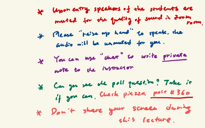
- . during share your screen Don 't * this lecture . - PowerPoint PPT Presentation

students Upon entry speakers of the are * for the quality of sound in Zoom muted room . ' ' raise up ' ' speak , the hand to Please * an muted for you will be audio . write private ' ' chat " to You can use * instructor the note to the poll question ? T ake it Can you see * post # 360 check piazza if can you - . during share your screen Don 't * this lecture .

Probability*and*Statistics* � ! for*Computer*Science** cov ( X, Y ) = E [( X − E [ X ])( Y − E [ Y ])] Covariance!is!coming!back!in! matrix! ! Credit:!wikipedia! Hongye!Liu,!Teaching!Assistant!Prof,!CS361,!UIUC,!03.25.2020!

Last*time* � Review!of!Maximum!likelihood! EsOmaOon!(MLE)! � Bayesian!Inference!(MAP)! videos Check out the discussion the pdf MLE for file and

Content* � Review!of!Bayesian!inference! � Visualizing!high!dimensional!data!&! Summarizing!data! � Refresh!of!some!linear!algebra! � The!covariance!matrix! !

Bayesian inference for p COLD ) O is . a probability distribution It is . Maximum Likely hood function a probability function is ( ( O ) =p ( DIO ) distribution . but NOT a Plot D) =PcDo , Bayes .e PID ) Rule

Beta%distribution% � A"distribu&on"is"Beta"distribu&on"if"it"has"the"following" expressive ! pdf:" P ( θ ) = K ( α , β ) θ α − 1 (1 − θ ) β − 1 OGG , I ] T T T " T ' , Boo 270 pdf of Beta − distribution K ( α , β ) = Γ ( α + β ) 10 Beta(1,1) Beta(5,5) "" Beta(50,50) Γ ( α ) Γ ( β ) Beta(70,70) Beta(20,50) 8 Beta(0.5,0.5) - � Is"an"expressive"family"of" 6 density distribu&ons""""""""""""""""""""""""""" Kisiel g 4 t � """"""""""""""""""""""""""""""is"uniform" Beta ( α = 1 , β = 1) 2 INFO to - x . 0 Ct k → 0.0 0.2 0.4 0.6 0.8 1.0 t ' a θ" . X

Beta%distribution%as%the%conjugate%prior% for%Binomial%likelihood% � The$likelihood$is$Binomial$( N ,$ k )$ � N � θ k (1 − θ ) N − k P ( D | θ ) = k � The$Beta$distribuOon$is$used$as$the$prior$ O C- Co , I ) P ( θ ) = K ( α , β ) θ α − 1 (1 − θ ) β − 1 " otherwise Pl 01=0 , � So$ P ( θ | D ) ∝ θ α + k − 1 (1 − θ ) β + N − k − 1 * � Then$the$posterior$is$$ Beta ( α + k, β + N − k ) P ( θ | D ) = K ( α + k, β + N − k ) θ α + k − 1 (1 − θ ) β + N − k − 1 Deco , I ]

The posterior for this example Continuous distribution Beta , is PCOID ) a - K - i c , - o , Btn " " C O is the X , , ] OGG random variable Binomial Distribution i r e Discrete Pl X -14=17 N - K , ) ok :c , - o , / the is K K 70 random why PLOID ) variable is not Binomial ?

The%update%of%Bayesian%posterior% � Since$the$posterior$is$in$the$same$family$as$the$ conjugate$prior,$the$posterior$can$be$used$as$a$new$prior$ if$more$data$is$observed.$ � Suppose$we$start$with$a$uniform$prior$on$the$ probability$θ$of$heads$ N" k" α" β" 1$ 1$ 3$ 0$ 1$ 4$ 10$ 7$ 8$ 7$ 30$ 17$ 25$ 20$ 100$ 72$ 97$ 48$ θ$

Maximize%the%Bayesian%posterior%(MAP)% � The$posterior$of$the$previous$example$is$ $ P ( θ | D ) = K ( α + k, β + N − k ) θ α + k − 1 (1 − θ ) β + N − k − 1 � DifferenOaOng$and$se^ng$to$0$gives$the$MAP$esOmate$ 2=1 α − 1 + k ˆ θ = B. =L α + β − 2 + N 1St prior - It 96 I 0<67 = - It I -2-1143

Conjugate%prior%for%other%likelihood% functions% � What$is$the$the$conjugate$prior$if$the$likelihood$is$ Bernoulli$or$geometric?$ Berta � What$is$the$the$conjugate$prior$if$the$likelihood$is$ Poisson$or$ExponenOal?$ Gamma � What$is$the$the$conjugate$prior$if$the$likelihood$is$ normal$with$known$variance?$ Normal

Content% � Review$of$Bayesian$inference$ � Visualizing"high"dimensional"data" &"Summarizing"data" � Refresh$of$some$linear$algebra$ � The$covariance$matrix$ $

A%data%set%with%7%dimensions% � Seed$data$set$from$the$UCI$Machine$Learning$ - site:$ - areaA$ perimeterP$ compactness$ lengthKernel$ widthKernel$ asymmetry$ lengthGroove$ Label$ - 15.26$ 14.84$ 0.871$ 5.763$ 3.312$ 2.221$ 5.22$ 1$ 1$ 14.88$ 14.57$ 0.8811$ 5.554$ 3.333$ 1.018$ 4.956$ 1$ 2$ 14.29$ 14.09$ 0.905$ 5.291$ 3.337$ 2.699$ 4.825$ 1$ 3$ 13.84$ 13.94$ 0.8955$ 5.324$ 3.379$ 2.259$ 4.805$ 1$ 4$ 16.14$ 14.99$ 0.9034$ 5.658$ 3.562$ 1.355$ 5.175$ 1$ 5$ 14.38$ 14.21$ 0.8951$ 5.386$ 3.312$ 2.462$ 4.956$ 1$ 6$ 14.69$ 14.49$ 0.8799$ 5.563$ 3.259$ 3.586$ 5.219$ 1$ 7$ …$

Matrix%format%of%a%dataset%in%the%textbook% N Co l - - - l - ! ) row :-p ← area A : : q , µ # of features d-