Document and Topic Models: pLSA and LDA Andrew Levandoski and - - PDF document

10/4/2018 1

Document and Topic Models: pLSA and LDA

Andrew Levandoski and Jonathan Lobo CS 3750 Advanced Topics in Machine Learning 2 October 2018

Outline

• Topic Models
• pLSA
• LSA
• Model
• Fitting via EM
• pHITS: link analysis
• LDA
• Dirichlet distribution
• Generative process
• Model
• Geometric Interpretation
• Inference

2

10/4/2018 2

Topic Models: Visual Representation

Topics Documents Topic proportions and assignments

3

Topic Models: Importance

• For a given corpus, we learn two things:
• 1. Topic: from full vocabulary set, we learn important subsets
• 2. Topic proportion: we learn what each document is about
• This can be viewed as a form of dimensionality reduction
• From large vocabulary set, extract basis vectors (topics)
• Represent document in topic space (topic proportions)
• Dimensionality is reduced from 𝑥𝑗 ∈ ℤ𝑊

𝑂 to 𝜄 ∈ ℝ𝐿

• Topic proportion is useful for several applications including document

classification, discovery of semantic structures, sentiment analysis,

• bject localization in images, etc.

4

10/4/2018 3

Topic Models: Terminology

• Document Model
• Word: element in a vocabulary set
• Document: collection of words
• Corpus: collection of documents
• Topic Model
• Topic: collection of words (subset of vocabulary)
• Document is represented by (latent) mixture of topics
• 𝑞 𝑥 𝑒 = 𝑞 𝑥 𝑨 𝑞(𝑨|𝑒) (𝑨 : topic)
• Note: document is a collection of words (not a sequence)
• ‘Bag of words’ assumption
• In probability, we call this the exchangeability assumption
• 𝑞 𝑥1, … , 𝑥𝑂 = 𝑞(𝑥𝜏 1 , … , 𝑥𝜏 𝑂 ) (𝜏: permutation)

5

Topic Models: Terminology (cont’d)

• Represent each document as a vector space
• A word is an item from a vocabulary indexed by {1, … , 𝑊}. We

represent words using unit‐basis vectors. The 𝑤𝑢ℎ word is represented by a 𝑊 vector 𝑥 such that 𝑥𝑤 = 1 and 𝑥𝑣 = 0 for 𝑤 ≠ 𝑣.

• A document is a sequence of 𝑜 words denoted by w = (𝑥1, 𝑥2, … 𝑥𝑜)

where 𝑥𝑜 is the nth word in the sequence.

• A corpus is a collection of 𝑁 documents denoted by

𝐸 = 𝑥1, 𝑥2, … 𝑥𝑛 .

6

10/4/2018 4

Probabilistic Latent Semantic Analysis (pLSA)

7

Motivation

• Learning from text and natural language
• Learning meaning and usage of words without prior linguistic

knowledge

• Modeling semantics
• Account for polysems and similar words
• Difference between what is said and what is meant

8

10/4/2018 5

Vector Space Model

• Want to represent documents and terms as vectors in a lower-

dimensional space

• N × M word-document co-occurrence matrix 𝜩
• limitations: high dimensionality, noisy, sparse
• solution: map to lower-dimensional latent semantic space using SVD

𝐸 = {𝑒1, . . . , 𝑒𝑂} W = {𝑥1, . . . , 𝑥𝑁} 𝜩 = 𝑜 𝑒𝑗, 𝑥

𝑘 𝑗𝑘

9

Latent Semantic Analysis (LSA)

• Goal
• Map high dimensional vector space representation to lower dimensional

representation in latent semantic space

• Reveal semantic relations between documents (count vectors)
• SVD
• N = UΣVT
• U: orthogonal matrix with left singular vectors (eigenvectors of NNT)
• V: orthogonal matrix with right singular vectors (eigenvectors of NTN)
• Σ: diagonal matrix with singular values of N
• Select k largest singular values from Σ to get approximation ෩

𝑂 with minimal error

• Can compute similarity values between document vectors and term vectors

10

10/4/2018 6

LSA

11

LSA Strengths

• Outperforms naïve vector space model
• Unsupervised, simple
• Noise removal and robustness due to dimensionality reduction
• Can capture synonymy
• Language independent
• Can easily perform queries, clustering, and comparisons

12

10/4/2018 7

LSA Limitations

• No probabilistic model of term occurrences
• Results are difficult to interpret
• Assumes that words and documents form a joint Gaussian model
• Arbitrary selection of the number of dimensions k
• Cannot account for polysemy
• No generative model

13

Probabilistic Latent Semantic Analysis (pLSA)

• Difference between topics and words?
• Words are observable
• Topics are not, they are latent
• Aspect Model
• Associates an unobserved latent class variable 𝑨 𝜗 ℤ = {𝑨1, . . . , 𝑨𝐿} with each
• bservation
• Defines a joint probability model over documents and words
• Assumes w is independent of d conditioned on z
• Cardinality of z should be much less than than d and w

14

10/4/2018 8

pLSA Model Formulation

• Basic Generative Model
• Select document d with probability P(d)
• Select a latent class z with probability P(z|d)
• Generate a word w with probability P(w|z)
• Joint Probability Model

𝑄 𝑒, 𝑥 = 𝑄 𝑒 𝑄 𝑥 𝑒 𝑄 𝑥|𝑒 = ෍

𝑨 𝜗 ℤ

𝑄 𝑥|𝑨 𝑄 𝑨 𝑒

15

pLSA Graphical Model Representation

16

𝑄 𝑒, 𝑥 = 𝑄 𝑒 𝑄 𝑥 𝑒 𝑄 𝑥|𝑒 = ෍

𝑨 𝜗 ℤ

𝑄 𝑥|𝑨 𝑄 𝑨 𝑒 𝑄 𝑒, 𝑥 = ෍

𝑨 𝜗 ℤ

𝑄 𝑨 𝑄 𝑒 𝑨 𝑄(𝑥|𝑨)

10/4/2018 9

pLSA Joint Probability Model

𝑄 𝑒, 𝑥 = 𝑄 𝑒 𝑄 𝑥 𝑒 𝑄 𝑥|𝑒 = ෍

𝑨 𝜗 ℤ

𝑄 𝑥|𝑨 𝑄 𝑨 𝑒 ℒ = ෍

𝑒𝜗𝐸

෍

𝑥𝜗𝑋

𝑜 𝑒, 𝑥 log 𝑄(𝑒, 𝑥) Maximize:

Corresponds to a minimization of KL divergence (cross-entropy) between the empirical distribution

• f words and the model distribution P(w|d)

17

Probabilistic Latent Semantic Space

• P(w|d) for all documents is

approximated by a multinomial combination of all factors P(w|z)

• Weights P(z|d) uniquely define a

point in the latent semantic space, represent how topics are mixed in a document

18

10/4/2018 10

Probabilistic Latent Semantic Space

• Topic represented by probability distribution over words
• Document represented by probability distribution over topics

19

𝑨𝑗 = (𝑥1, . . . , 𝑥𝑛) 𝑨1 = (0.3, 0.1, 0.2, 0.3, 0.1) 𝑒𝑘 = (𝑨1, . . . , 𝑨𝑜) 𝑒1 = (0.5, 0.3, 0.2)

Model Fitting via Expectation Maximization

• E-step
• M-step

𝑄 𝑨 𝑒, 𝑥 = 𝑄 𝑨 𝑄 𝑒 𝑨 𝑄 𝑥 𝑨 σ𝑨′ 𝑄 𝑨′ 𝑄 𝑒 𝑨′ 𝑄(𝑥|𝑨′) 𝑄(𝑥|𝑨) = σ𝑒 𝑜 𝑒, 𝑥 𝑄(𝑨|𝑒, 𝑥) σ𝑒,𝑥′ 𝑜 𝑒, 𝑥′ 𝑄(𝑨|𝑒, 𝑥′) 𝑄(𝑒|𝑨) = σ𝑥 𝑜 𝑒, 𝑥 𝑄(𝑨|𝑒, 𝑥) σ𝑒′,𝑥 𝑜 𝑒′, 𝑥 𝑄(𝑨|𝑒′, 𝑥) 𝑄 𝑨 = 1 𝑆 ෍

𝑒,𝑥

𝑜 𝑒, 𝑥 𝑄 𝑨 𝑒, 𝑥 , 𝑆 ≡ ෍

𝑒,𝑥

𝑜(𝑒, 𝑥) Compute posterior probabilities for latent variables z using current parameters Update parameters using given posterior probabilities

20

10/4/2018 11

pLSA Strengths

• Models word-document co-occurrences as a mixture of conditionally

independent multinomial distributions

• A mixture model, not a clustering model
• Results have a clear probabilistic interpretation
• Allows for model combination
• Problem of polysemy is better addressed

21

pLSA Strengths

• Problem of polysemy is better addressed

22

10/4/2018 12

pLSA Limitations

• Potentially higher computational complexity
• EM algorithm gives local maximum
• Prone to overfitting
• Solution: Tempered EM
• Not a well defined generative model for new documents
• Solution: Latent Dirichlet Allocation

23

pLSA Model Fitting Revisited

• Tempered EM
• Goals: maximize performance on unseen data, accelerate fitting process
• Define control parameter β that is continuously modified
• Modified E-step

𝑄𝛾 𝑨 𝑒, 𝑥 = 𝑄 𝑨 𝑄 𝑒 𝑨 𝑄 𝑥 𝑨

𝛾

σ𝑨′ 𝑄 𝑨′ 𝑄 𝑒 𝑨′ 𝑄 𝑥 𝑨′

𝛾

24

10/4/2018 13

Tempered EM Steps

1) Split data into training and validation sets 2) Set β to 1 3) Perform EM on training set until performance on validation set decreases 4) Decrease β by setting it to ηβ, where η <1, and go back to step 3 5) Stop when decreasing β gives no improvement

25

Example: Identifying Authoritative Documents

26

10/4/2018 14

HITS

• Hubs and Authorities
• Each webpage has an authority score x and a hub score y
• Authority – value of content on the page to a community
• likelihood of being cited
• Hub – value of links to other pages
• likelihood of citing authorities
• A good hub points to many good authorities
• A good authority is pointed to by many good hubs
• Principal components correspond to different communities
• Identify the principal eigenvector of co-citation matrix

27

HITS Drawbacks

• Uses only the largest

eigenvectors, not necessary the

• nly relevant communities
• Authoritative documents in

smaller communities may be given no credit

• Solution: Probabilistic HITS

28

10/4/2018 15

pHITS

𝑄 𝑒, 𝑑 = ෍

𝑨

𝑄 𝑨 𝑄 𝑑 𝑨 𝑄(𝑒|𝑨)

P(d|z) P(c|z)

Documents Communities

Citations

29

Interpreting pHITS Results

• Explain d and c in terms of the latent variable “community”
• Authority score: P(c|z)
• Probability of a document being cited from within community z
• Hub Score: P(d|z)
• Probability that a document d contains a reference to community z.
• Community Membership: P(z|c).
• Classify documents

30

10/4/2018 16

Joint Model of pLSA and pHITS

• Joint probabilistic model of document content (pLSA) and

connectivity (pHITS)

• Able to answer questions on both structure and content
• Model can use evidence about link structure to make predictions about

document content, and vice versa

• Reference flow – connection between one topic and another
• Maximize log-likelihood function

ℒ = ෍

𝑘

𝛽 ෍

𝑗

𝑂𝑗𝑘 σ𝑗′ 𝑂𝑗′𝑘 𝑚𝑝𝑕 ෍

𝑙

𝑄 𝑥𝑗 𝑨𝑙 𝑄 𝑨𝑙 𝑒𝑘 + (1 − 𝛽) ෍

𝑚

𝐵𝑚𝑘 σ𝑚′ 𝐵𝑚′𝑘 𝑚𝑝𝑕 ෍

𝑙

𝑄 𝑑𝑚 𝑨𝑙 𝑄 𝑨𝑙 𝑒𝑘

31

pLSA: Main Deficiencies

• Incomplete in that it provides no probabilistic model at the document level

i.e. no proper priors are defined.

• Each document is represented as a list of numbers (the mixing proportions

for topics), and there is no generative probabilistic model for these numbers, thus:

• 1. The number of parameters in the model grows linearly with the size of the

corpus, leading to overfitting

• 2. It is unclear how to assign probability to a document outside of the training set
• Latent Dirichlet allocation (LDA) captures the exchangeability of both

words and documents using a Dirichlet distribution, allowing a coherent generative process for test data

32

10/4/2018 17

Latent Dirichlet Allocation (LDA)

33

LDA: Dirichlet Distribution

34

• A ‘distribution of distributions’
• Multivariate distribution whose components all take values on

(0,1) and which sum to one.

• Parameterized by the vector α, which has the same number of

elements (k) as our multinomial parameter θ.

• Generalization of the beta distribution into multiple dimensions
• The alpha hyperparameter controls the mixture of topics for a

given document

• The beta hyperparameter controls the distribution of words per

topic Note: Ideally we want our composites to be made up of only a few topics and our parts to belong to only some of the topics. With this in mind, alpha and beta are typically set below one.

10/4/2018 18

LDA: Dirichlet Distribution (cont’d)

• A k-dimensional Dirichlet random variable 𝜄 can take values in the (k-

1)-simplex (a k-vector 𝜄 lies in the (k-1)-simplex if 𝜄𝑗 ≥ 0, σ𝑗=1

𝑙

𝜄𝑗 = 1) and has the following probability density on this simplex: 𝑞 𝜄 𝛽 =

Γ(σ𝑗=1

𝑙

𝛽𝑗) ς𝑗=1

𝑙

Γ(𝛽𝑗) 𝜄1 𝛽1−1 … 𝜄𝑙 𝛽𝑙−1,

where the parameter 𝛽 is a k-vector with components 𝛽𝑗 > 0 and where Γ(𝑦) is the Gamma function.

• The Dirichlet is a convenient distribution on the simplex:
• In the exponential family
• Has finite dimensional sufficient statistics
• Conjugate to the multinomial distribution

35

LDA: Generative Process

LDA assumes the following generative process for each document 𝑥 in a corpus 𝐸:

• 1. Choose 𝑂 ~ 𝑄𝑝𝑗𝑡𝑡𝑝𝑜 𝜊 .
• 2. Choose 𝜄 ~ 𝐸𝑗𝑠 𝛽 .
• 3. For each of the 𝑂 words 𝑥𝑂:

a. Choose a topic 𝑨𝑜 ~ 𝑁𝑣𝑚𝑢𝑗𝑜𝑝𝑛𝑗𝑏𝑚 𝜄 . b. Choose a word 𝑥𝑜 from 𝑞(𝑥𝑜|𝑨𝑜, 𝛾), a multinomial probability conditioned on the topic 𝑨𝑜.

Example: Assume a group of articles that can be broken down by three topics described by the following words:

• Animals: dog, cat, chicken, nature, zoo
• Cooking: oven, food, restaurant, plates, taste
• Politics: Republican, Democrat, Congress, ineffective, divisive

To generate a new document that is 80% about animals and 20% about cooking:

• Choose the length of the article (say, 1000 words)
• Choose a topic based on the specified mixture (~800 words will coming from topic ‘animals’)
• Choose a word based on the word distribution for each topic

36

10/4/2018 19

LDA: Model (Plate Notation)

𝛽 is the parameter of the Dirichlet prior on the per-document topic distribution, 𝛾 is the parameter of the Dirichlet prior on the per-topic word distribution, 𝜄𝑁 is the topic distribution for document M, 𝑨𝑁𝑂 is the topic for the N-th word in document M, and 𝑥𝑁𝑂 is the word.

37

LDA: Model

38

Parameters of Dirichlet distribution (K-vector)

dk dn ki dn d

𝜄𝑒𝑙 𝑨𝑒𝑜 = {1, … , 𝐿} 𝛾𝑙𝑗 = 𝑞(𝑥|𝑨)

1 … topic … K 1 … nth word … Nd 1 … word idx … V 1 ⋮ doc ⋮ M 1 ⋮ doc ⋮ M 1 ⋮ topic ⋮ M

10/4/2018 20

LDA: Model (cont’d)

39

controls the mixture of topics controls the distribution of words per topic

LDA: Model (cont’d)

Given the parameters 𝛽 and 𝛾, the joint distribution of a topic mixture 𝜄, a set of 𝑂 topics 𝑨, and a set of 𝑂 words 𝑥 is given by:

𝑞 𝜄, 𝑨, 𝑥 𝛽, 𝛾 = 𝑞 𝜄 𝛽 ෑ

𝑜=1 𝑂

𝑞 𝑨𝑜 𝜄 𝑞 𝑥𝑜 𝑨𝑜, 𝛾 ,

where 𝑞 𝑨𝑜 𝜄 is 𝜄𝑗 for the unique 𝑗 such that 𝑨𝑜

𝑗 = 1. Integrating over 𝜄 and summing over 𝑨, we obtain

the marginal distribution of a document:

𝑞 𝑥 𝛽, 𝛾 = න 𝑞(𝜄|𝛽) ෑ

𝑜=1 𝑂

෍

𝑨𝑜

𝑞 𝑨𝑜 𝜄 𝑞(𝑥𝑜|𝑨𝑜, 𝛾) 𝑒𝜄𝑒.

Finally, taking the products of the marginal probabilities of single documents, we obtain the probability of a corpus:

𝑞 𝐸 𝛽, 𝛾 = ෑ

𝑒=1 𝑁

න 𝑞(𝜄𝑒|𝛽) ෑ

𝑜=1 𝑂𝑒

෍

𝑨𝑒𝑜

𝑞 𝑨𝑒𝑜 𝜄𝑒 𝑞(𝑥𝑒𝑜|𝑨𝑒𝑜, 𝛾) 𝑒𝜄𝑒.

40

10/4/2018 21

LDA: Exchangeability

• A finite set of random variables {𝑦1, … , 𝑦𝑂} is said to be exchangeable if the

joint distribution is invariant to permutation. If π is a permutation of the integers from 1 to N: 𝑞 𝑦1, … , 𝑦𝑂 = 𝑞(𝑦𝜌1, … , 𝑦𝜌𝑂)

• An infinite sequence of random numbers is infinitely exchangeable if every

finite sequence is exchangeable

• We assume that words are generated by topics and that those topics are

infinitely exchangeable within a document

• By De Finetti’s Theorem:

𝑞 𝑥, 𝑨 = න 𝑞(𝜄) ෑ

𝑜=1 𝑂

𝑞 𝑨𝑜 𝜄 𝑞(𝑥𝑜|𝑨𝑜) 𝑒𝜄

41

LDA vs. other latent variable models

42

Unigram model: 𝑞 𝑥 = ς𝑜=1

𝑂

𝑞(𝑥𝑜) Mixture of unigrams: 𝑞 𝑥 = σ𝑨 𝑞(𝑨) ς𝑜=1

𝑂

𝑞(𝑥𝑜|𝑨) pLSI: 𝑞 𝑒, 𝑥𝑜 = 𝑞(𝑒) σ𝑨 𝑞 𝑥𝑜 𝑨 𝑞(𝑨|𝑒)

10/4/2018 22

LDA: Geometric Interpretation

43

• Topic simplex for three topics embedded

in the word simplex for three words

• Corners of the word simplex correspond to

the three distributions where each word has probability one

• Corners of the topic simplex correspond to

three different distributions over words

• Mixture of unigrams places each

document at one of the corners of the topic simplex

• pLSI induces an empirical distribution on

the topic simplex denoted by diamonds

• LDA places a smooth distribution on the

topic simplex denoted by contour lines

LDA: Goal of Inference

LDA inputs: Set of words per document for each document in a corpus LDA outputs: Corpus-wide topic vocabulary distributions Topic assignments per word Topic proportions per document

44

?

10/4/2018 23

LDA: Inference

45

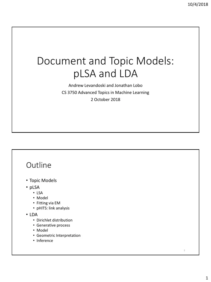
The key inferential problem we need to solve with LDA is that of computing the posterior distribution

• f the hidden variables given a document:

𝑞 𝜄, 𝑨 𝑥, 𝛽, 𝛾 = 𝑞(𝜄, 𝑨, 𝑥|𝛽, 𝛾) 𝑞(𝑥|𝛽, 𝛾) This formula is intractable to compute in general (the integral cannot be solved in closed form), so to normalize the distribution we marginalize over the hidden variables: 𝑞 𝑥 𝛽, 𝛾 = Γ(σ𝑗 𝛽𝑗) ς𝑗 Γ(𝛽𝑗) න ෑ

𝑗=1 𝑙

𝜄𝑗

𝛽𝑗−1

ෑ

𝑜=1 𝑂

෍

𝑗=1 𝑙

ෑ

𝑘=1 𝑊

(𝜄𝑗𝛾𝑗𝑘)𝑥𝑜

𝑘

𝑒𝜄

LDA: Variational Inference

• Basic idea: make use of Jensen’s inequality to obtain an adjustable lower

bound on the log likelihood

• Consider a family of lower bounds indexed by a set of variational

parameters chosen by an optimization procedure that attempts to find the tightest possible lower bound

• Problematic coupling between 𝜄 and 𝛾 arises due to edges between 𝜄, z

and w. By dropping these edges and the w nodes, we obtain a family of distributions on the latent variables characterized by the following variational distribution: 𝑟 𝜄, 𝑨 𝛿, 𝜚 = 𝑟 𝜄 𝛿 ෑ

𝑜=1 𝑂

𝑟 𝑨𝑜 𝜚𝑜 where 𝛿 and (𝜚1, … , 𝜚𝑜) and the free variational parameters.

46

10/4/2018 24

LDA: Variational Inference (cont’d)

• With this specified family of probability distributions, we set up the following
• ptimization problem to determine 𝜄 and 𝜚:

𝛿∗, 𝜚∗ = 𝑏𝑠𝑕𝑛𝑗𝑜 𝛿,𝜚 𝐸(𝑟(𝜄, 𝑨|𝛿, 𝜚) ∥ 𝑞 𝜄, 𝑨 𝑥, 𝛽, 𝛾 )

• The optimizing values of these parameters are found by minimizing the KL divergence

between the variational distribution and the true posterior 𝑞 𝜄, 𝑨 𝑥, 𝛽, 𝛾

• By computing the derivatives of the KL divergence and setting them equal to zero, we
• btain the following pair of update equations:

𝜚𝑜𝑗 ∝ 𝛾𝑗𝑥𝑜 exp 𝐹𝑟 log 𝜄𝑗 𝛿 𝛿𝑗 = 𝛽𝑗 + ෍

𝑜=1 𝑂

𝜚𝑜𝑗

• The expectation in the multinomial update can be computed as follows:

𝐹𝑟 log 𝜄𝑗 𝛿 = Ψ 𝛿𝑗 − Ψ(ෑ

𝑘=1 𝑙

𝛿𝑘) where Ψ is the first derivative of the logΓ function.

47

LDA: Variational Inference (cont’d)

48

10/4/2018 25

LDA: Parameter Estimation

• Given a corpus of documents 𝐸 = {𝑥1, 𝑥2 … , 𝑥𝑁}, we wish to find 𝛽

and 𝛾 that maximize the marginal log likelihood of the data: ℓ 𝛽, 𝛾 = ෍

𝑒=1 𝑁

𝑚𝑝𝑕𝑞(𝑥𝑒|𝛽, 𝛾)

• Variational EM yields the following iterative algorithm:

1. (E-step) For each document, find the optimizing values of the variational parameters 𝛿𝑒

∗, 𝜚𝑒 ∗: 𝑒 ∈ 𝐸

2. (M-step) Maximize the resulting lower bound on the log likelihood with respect to the model parameters 𝛽 and 𝛾

These two steps are repeated until the lower bound on the log likelihood converges.

49

LDA: Smoothing

50

• Introduces Dirichlet smoothing on 𝛾 to

avoid the zero frequency word problem

• Fully Bayesian approach:

𝑟 𝛾1:𝑙, 𝑨1:𝑁, 𝜄1:𝑁 𝜇, 𝜚, 𝛿 = ෍

𝑗=1 𝑙

𝐸𝑗𝑠(𝛾𝑗|𝜇𝑗) ෑ

𝑒=1 𝑁

𝑟𝑒(𝜄𝑒, 𝑨𝑒|𝜚𝑒, 𝛿𝑒) where 𝑟𝑒(𝜄, 𝑨 |𝜚, 𝛿) is the variational distribution defined for LDA. We require an additional update for the new variational parameter 𝜇: 𝜇𝑗𝑘 = 𝜃 + ෍

𝑒=1 𝑁

෍

𝑜=1 𝑂𝑒

𝜚𝑒𝑜𝑗

∗

𝑥𝑒𝑜

𝑘

10/4/2018 26

Topic Model Applications

• Information Retrieval
• Visualization
• Computer Vision
• Document = image, word = “visual word”
• Bioinformatics
• Genomic features, gene sequencing, diseases
• Modeling networks
• cities, social networks

51

pLSA / LDA Libraries

• gensim (Python)
• MALLET (Java)
• topicmodels (R)
• Stanford Topic Modeling Toolbox

10/4/2018 27

References

David M. Blei, Andrew Y. Ng, Michael I. Jordan. Latent Dirichlet Allocation. JMLR, 2003. David Cohn and Huan Chang. Learning to probabilistically identify Authoritative

• documents. ICML, 2000.

David Cohn and Thomas Hoffman. The Missing Link - A Probabilistic Model of Document Content and Hypertext Connectivity. NIPS, 2000. Thomas Hoffman. Probabilistic Latent Semantic Analysis. UAI-99, 1999. Thomas Hofmann. Probabilistic Latent Semantic Indexing. SIGIR-99, 1999.

53