Distance-Time Graphs MPM1D: Principles of Mathematics A - - PDF document

a n a l y z i n g d a t a

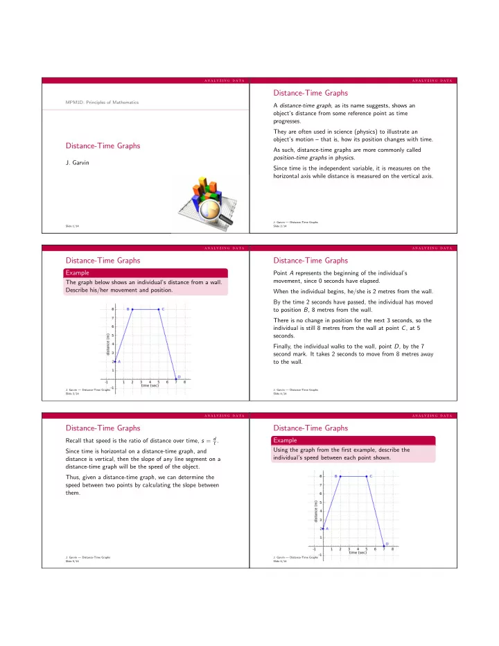
MPM1D: Principles of Mathematics

Distance-Time Graphs

• J. Garvin

Slide 1/14

a n a l y z i n g d a t a

Distance-Time Graphs

A distance-time graph, as its name suggests, shows an

• bject’s distance from some reference point as time

progresses. They are often used in science (physics) to illustrate an

• bject’s motion – that is, how its position changes with time.

As such, distance-time graphs are more commonly called position-time graphs in physics. Since time is the independent variable, it is measures on the horizontal axis while distance is measured on the vertical axis.

• J. Garvin — Distance-Time Graphs

Slide 2/14

a n a l y z i n g d a t a

Distance-Time Graphs

Example

The graph below shows an individual’s distance from a wall. Describe his/her movement and position.

• J. Garvin — Distance-Time Graphs

Slide 3/14

a n a l y z i n g d a t a

Distance-Time Graphs

Point A represents the beginning of the individual’s movement, since 0 seconds have elapsed. When the individual begins, he/she is 2 metres from the wall. By the time 2 seconds have passed, the individual has moved to position B, 8 metres from the wall. There is no change in position for the next 3 seconds, so the individual is still 8 metres from the wall at point C, at 5 seconds. Finally, the individual walks to the wall, point D, by the 7 second mark. It takes 2 seconds to move from 8 metres away to the wall.

• J. Garvin — Distance-Time Graphs

Slide 4/14

a n a l y z i n g d a t a

Distance-Time Graphs

Recall that speed is the ratio of distance over time, s = d

t .

Since time is horizontal on a distance-time graph, and distance is vertical, then the slope of any line segment on a distance-time graph will be the speed of the object. Thus, given a distance-time graph, we can determine the speed between two points by calculating the slope between them.

• J. Garvin — Distance-Time Graphs

Slide 5/14

a n a l y z i n g d a t a

Distance-Time Graphs

Example

Using the graph from the first example, describe the individual’s speed between each point shown.

• J. Garvin — Distance-Time Graphs

Slide 6/14

a n a l y z i n g d a t a

Distance-Time Graphs

It takes 2 seconds to travel from point A to B, a change from 2 metres to 8 metres. The slope of this segment is m = 8−2

2−0 = 3. Therefore, the

individual’s speed is 3 m/s. Since the segment from B to C is horizontal, it has a slope

• f zero. Therefore, for the 3 seconds between B and C, the

individual is motionless. To travel the 8 metres from C to D takes 2 seconds. Let this speed be negative, since the distance from the wall is decreasing. Therefore, the speed of the individual from C to D is m = 8−0

7−5 = −4 m/s.

• J. Garvin — Distance-Time Graphs

Slide 7/14

a n a l y z i n g d a t a

Distance-Time Graphs

Example

Use the graph below to interpret an individual’s position from a wall, and his/her speed.

• J. Garvin — Distance-Time Graphs

Slide 8/14

a n a l y z i n g d a t a

Distance-Time Graphs

The individual starts 5 metres from the wall, and stays motionless for 2 seconds. Over the next 3 seconds, the individual moves from 5 metres to 2 metres away from the wall. His/her speed is m = − 3

3 = −1 m/s.

The individual is motionless between 5 and 6 seconds. From 6 to 8 seconds, the individual walks toward the wall at a speed of − 2

2 = −1 m/s.

• J. Garvin — Distance-Time Graphs

Slide 9/14

a n a l y z i n g d a t a

Distance-Time Graphs

In the previous examples, all line segments were straight lines. While this is convenient, it is not entirely accurate. It takes time to speed up or slow down, so most “real life” distance-time graphs will be represented with curves connecting straighter segments. If a curve is getting steeper, an object’s speed is increasing, whereas if a curve is flattening out, its speed is decreasing.

• J. Garvin — Distance-Time Graphs

Slide 10/14

a n a l y z i n g d a t a

Distance-Time Graphs

Example

How does the speed of the object, whose position-time graph is shown, change with time?

• J. Garvin — Distance-Time Graphs

Slide 11/14

a n a l y z i n g d a t a

Distance-Time Graphs

Between points A and B, the curve changes from fairly steep to nearly flat. Thus, the speed of the object is decreasing from A to B. From B to C, the curve gets steeper, so the speed of the

• bject is increasing from B to C.

Since the line segment after point C is a straight line, this indicates a constant speed. Beyond point C, the speed of the object is neither increasing nor decreasing.

• J. Garvin — Distance-Time Graphs

Slide 12/14

a n a l y z i n g d a t a

Distance-Time Graphs

Example

Use the distance-time graph below to create a story of your

• wn.
• J. Garvin — Distance-Time Graphs

Slide 13/14

a n a l y z i n g d a t a

Questions?

• J. Garvin — Distance-Time Graphs

Slide 14/14