Discrete-Event Systems and Generalized Semi-Markov Processes - - PowerPoint PPT Presentation

Discrete-Event Systems and Generalized Semi-Markov Processes

Reading: Section 1.4 in Shedler or Section 4.1 in Haas Peter J. Haas CS 590M: Simulation Spring Semester 2020

1 / 27

Discrete-Event Systems and Generalized Semi-Markov Processes Discrete-Event Stochastic Systems The GSMP Model Simulating GSMPs Generating Clock Readings: Inversion Method Markovian and Semi-Markovian GSMPs

2 / 27

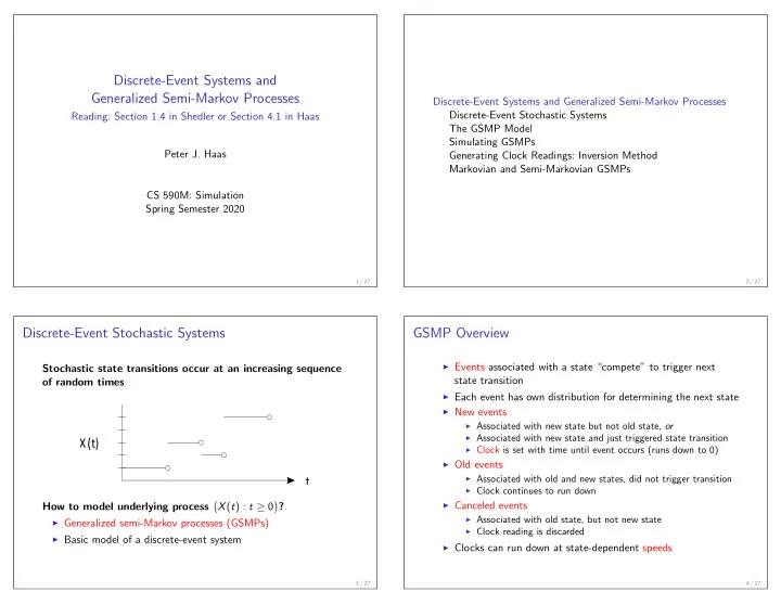
Discrete-Event Stochastic Systems

Stochastic state transitions occur at an increasing sequence

• f random times

t X(t)

How to model underlying process

• X(t) : t ≥ 0
• ?

◮ Generalized semi-Markov processes (GSMPs) ◮ Basic model of a discrete-event system

3 / 27

GSMP Overview

◮ Events associated with a state “compete” to trigger next

state transition

◮ Each event has own distribution for determining the next state ◮ New events

◮ Associated with new state but not old state, or ◮ Associated with new state and just triggered state transition ◮ Clock is set with time until event occurs (runs down to 0)

◮ Old events

◮ Associated with old and new states, did not trigger transition ◮ Clock continues to run down

◮ Canceled events

◮ Associated with old state, but not new state ◮ Clock reading is discarded

◮ Clocks can run down at state-dependent speeds

4 / 27

Clock-Reading Plot

5 / 27

GSMP Building Blocks

◮ S: a (finite or countably infinite) set of states ◮ E = {e1, e2, . . . , eM}: a finite set of events ◮ E(s) ⊆ E: the set of active events in state s ∈ S ◮ p(s′; s, E ∗): probability that new state = s′ when events in E ∗

simultaneously occur in s

◮ Write p(s′; s, e∗) if E ∗ = {e∗} (unique trigger event)

◮ r(s, e): the nonnegative finite speed at which clock for e runs

down in state s

◮ Typically r(s, e) = 1 ◮ Set r(s, e) = 0 to model “preempt resume” service discipline

◮ F( · ; s′, e′, s, E ∗): cdf of new clock-reading for e′ after state

transition s

E ∗

− → s′

◮ µ: initial distribution for state and clock readings

◮ Assume initial state s

D

∼ ν and clock readings

D

∼ F0( · ; e, s)

6 / 27

New and Old Events

7 / 27

Example: GI/G/1 Queue

• Assume that interarrival-time dist’n Fa and service-time

dist’n Fs are continuous (no simult. event occurrences)

• Assume that at time t = 0 a job arrives to an empty system

X(t) = # of jobs in service or waiting in queue at time t Can define (X(t) : t ≥ 0) as a GSMP:

◮ S = ◮ E = ◮ E(s) = ◮ p: ◮ F(x; s′, e′, s, e∗) : ◮ r(s, e) = ◮ Initial dist’n:

8 / 27

A More Complex Example: Patrolling Repairman

See handout for details

◮ Provides an example of how to concisely express GSMP

building blocks Specifying a GSMP can be complex and time-consuming, so why do it?

◮ Direct guidance for coding (helps catch “corner cases”) ◮ Communicates model at high level (vs poring through code) ◮ Theory for GSMPs can help in establishing important

properties of the simulation

◮ Stability (i.e., convergence to steady state), so that

steady-state estimation problems are well defined

◮ Validity of specific simulation output-analysis methods, so that

estimates are correct

9 / 27

GSMPs and GSSMCs

GSMP formally defined in terms of GSSMC

• (Sn, Cn) : n ≥ 0
• ◮ Sn = state just after nth transition

◮ Cn = (Cn,1, Cn,2, . . . , Cn,M) = clock readings just after nth

transition

◮ See Haas or Shedler books for definition of P

• (s, c), A
• and µ

10 / 27

GSMP Definition

Define

◮ Holding time: t∗(s, c) = min{i:ei∈E(s)} ci/r(s, ei) ◮ nth state-transition time: ζn = n−1 k=0 t∗(s, c) ◮ # of state transitions in [0, t]: N(t) = max{n ≥ 0 : ζn ≤ t}

Let ∆ ∈ S and set

X(t) =

• SN(t)

if N(t) < ∞; ∆ if N(t) = ∞

11 / 27

GSMP Definition in a Picture

ζ0 = 0 ζ1 S1 S0 S3 S2

t S C *( , ) t S C *( , )

1 1

t S C *( , )

2 2

ζ2 ζ3 ζ4 t

N t ( ) = 0 N t ( ) = 1 N t ( ) = 2 X t S ( ) = 3 N t ( ) = 3

t S C *( , )

3 3

12 / 27

Discrete-Event Systems and Generalized Semi-Markov Processes Discrete-Event Stochastic Systems The GSMP Model Simulating GSMPs Generating Clock Readings: Inversion Method Markovian and Semi-Markovian GSMPs

13 / 27

Sample Path Generation

GSMP Simulation Algorithm (Variable Time-Advance)

• 1. (Initialization) Select s D

∼ ν. For each ei ∈ E(s) generate a clock reading ci

D

∼ F0( · ; ei, s). Set ci = 0 for ei / ∈ E(s).

• 2. Determine holding time t∗(s, c) and set of trigger events

E ∗ = E ∗(s, c) = {ei : ci/r(s, ei) = t∗(s, c)}.

• 3. Generate next state s′ D

∼ p( · ; s, E ∗).

• 4. For each ei ∈ N(s′; s, E ∗), generate c′

i D

∼ F( · ; s′, ei, s, E ∗).

• 5. For each ei ∈ O(s′; s, E ∗), set c

′

i = ci − t∗(s, c) r(s, ei).

• 6. For each ei ∈ (E(s) − E ∗) − E(s′), set c′

i = 0

(i.e., cancel event ei).

• 7. Set s = s′ and c = c′, and go to Step 2.

(Here c = (c1, c2, . . . , cM) and similarly for c′.)

14 / 27

Sample Path Generation, Continued

Algorithm generates sequence of states (Sn : n ≥ 0), clock-reading vectors (Cn : n ≥ 0), and holding times

• t∗(Sn, Cn) : n ≥ 0
• Transition times (ζn : n ≥ 0) and continuous-time process
• X(n) : n ≥ 0
• computed as described previously

Use usual techniques to estimate quantities like E

• f
• X(t)
• r even

α = E 1 t t f

• X(u)
• du
• = E
• 1

t N(t)−1

• n=0

f (Sn)t∗(Sn, Cn) + f (SN(t))

• t − ζN(t)
• Flow charts and diagrams can be helpful

(see Law, p. 30–32 for an example)

15 / 27

Discrete-Event Systems and Generalized Semi-Markov Processes Discrete-Event Stochastic Systems The GSMP Model Simulating GSMPs Generating Clock Readings: Inversion Method Markovian and Semi-Markovian GSMPs

16 / 27

Generating Clock Readings: Example

Exponential distribution with rate (intensity) λ

f (x; λ) =

• λe−λx

if x ≥ 0; if x < 0 and F(x; λ) =

• 1 − e−λx

if x ≥ 0; if x < 0

Mean = 1/λ

Claim:

If U D ∼ Uniform(0, 1) and V = − ln U

λ

, then V D ∼ exp(λ) Proof:

17 / 27

The Inversion Method: Special Case

Spose that cdf F(x) = P(V ≤ x) is increasing and continuous

Claim:

If U D ∼ Uniform(0, 1) and V = F −1(U), then V D ∼ F Proof:

18 / 27

Example: Exponential Distribution

F(x) = 1 − e−λx F −1(u) =

19 / 27

The Inversion Method: General Case

Generalized inverse

F −1(u) = min{x : F(x) ≥ u} F(x) x

u F (u)

• 1

Claim still holds: F −1(u) ≤ x ⇔ u ≤ F(x) by definition Exercise: Show that inversion method = naive method for discrete RVs

20 / 27

Discrete-Event Systems and Generalized Semi-Markov Processes Discrete-Event Stochastic Systems The GSMP Model Simulating GSMPs Generating Clock Readings: Inversion Method Markovian and Semi-Markovian GSMPs

21 / 27

Markovian GSMPs

Properties of the Exponential Distribution

If X D ∼ exp(λ) and Y D ∼ exp(µ) then

• 1. min(X, Y ) D

∼ exp(λ + µ) [indep. of whether min = X or Y ]

• 2. P(X < Y ) =

λ λ+µ

• 3. P(X > a + b | X > a) = e−λb [memoryless property]

Properties 1 and 2 generalize to multiple exponential RVs

Simple GSMP event e′

F(· ; s′, e′, s, E ∗) ≡ F(· ; e′) and F0(· ; e′; s) ≡ F(· ; e′)

22 / 27

Markovian GSMPs, Continued

Suppose that all events in a GSMP are simple with exponential clock-setting distn’s Key observation: By memoryless property, whenever GSMP jumps into a state s, clock readings for events in E(s) are mutually independent and exponentially distributed

Simplified Simulation Algorithm (No clock readings needed)

• 1. (Initialization) Select s D

∼ ν

• 2. Generate holding time t∗ D

∼ exp(λ), where λ = λ(s) =

ei∈E(s) λi

• 3. Select ei ∈ E(s) as trigger event with probability λi/λ
• 4. Generate the next state s′ D

∼ p( · ; s, ei)

• 5. Set s = s′ and go to Step 2

23 / 27

Markovian GSMPs, Continued

Structure of a Markovian GSMP

◮ Sequence (Sn : n ≥ 0) is a DTMC with transition matrix

R(s, s′) =

ei∈E(s) p(s′; s, ei)(λi/λ) ◮ Given (Sn : n ≥ 0), holding times are mutually independent

with holding time in Sn

D

∼ exp

• λ(Sn)
• Often, occurrence of ei in s causes state to change to a

unique state yi = yi(s) with probability 1

Super-Simplified Simulation Algorithm

• 1. (Initialization) Select s D

∼ ν

• 2. Generate holding time t∗ D

∼ exp(λ), where λ =

ei∈E(s) λi

• 3. Set s′ = yi(s) with probability λi/λ
• 4. Set s = s′ and go to Step 2

24 / 27

Markovian GSMPs, Continued

A GSMP

• X(t) : t ≥ 0)
• with simple, exponential transitions

is a continuous-time Markov chain (CTMC) [Ross, Ch. 6]

◮ Finite or countable state space ◮ Continuous-time Markov property

P

• X(t + u) = s | X(s) : 0 ≤ s ≤ t
• = P
• X(t + u) = s | X(t)
• All CTMCs have foregoing structure

◮ State sequence is a DTMC ◮ Holding times mutually independent and exp

• λ(s)
• in state s

Q: What can go wrong if events are not simple?

25 / 27

Example of Markovian GSMP: Poisson Process

Definition of Poisson process

• N(t) : t ≥ 0
• with rate λ

◮ S = {0, 1, 2, . . .} ◮ Single exp(λ) event ◮ p(s + 1; s, e) = 1

Can show that

P

• N(t + s) = m + n | N(t) = m
• = e-λs(λs)n

n!

Examples: # arrivals to a queue, # of lightbulb replacements

26 / 27

Semi-Markovian GSMPs

GSMP

• X(t) : t ≥ 0
• with simple events such that |E(s)| = 1

for all s ∈ S is a semi-Markov process Definition of semi-Markov process

◮ Discrete state space S ◮ State sequence (Xn : n ≥ 0) is a DTMC with transition

matrix, say, R

◮ Holding time in s D

∼ F( · ; s)

◮ “Markov property holds only at state-transition times”

Example: Renewal counting process

◮ S = {0, 1, 2, . . .} ◮ R(s, s + 1) = 1 for all s ∈ S ◮ F( · ; s) ≡ G( · ) for some G

27 / 27