Dichotomies and Growth Function Matthieu R. Bloch 1 Motivation For - - PDF document

ECE 6254 - Spring 2020 - Lecture 16 v1.0 - revised March 24, 2020

Dichotomies and Growth Function

Matthieu R. Bloch

1 Motivation For a hypothesis set H with |H| = M and h∗ = argmaxh∈H

RN(h), we have shown earlier that ∀ϵ > 0 P

• RN(h∗) − R(h∗)
• ⩾ ϵ
• ⩽ 2M exp(−2Nϵ2).

(1) In particular, the factor M is the result of the union bound, which we used to show that for ϵ > 0 P

• RN(h∗) − R(h∗)
• ⩾ ϵ
• ⩽ P
• max

h∈H

• RN(h) − R(h)
• ⩾ ϵ
• (2)

⩽

M

• j=1

P

• RN(hj) − R(hj)
• ⩾ ϵ
• .

(3) Tie second inequality is tight when the events Ej ≜ {

• RN(hj) − R(hj)
• ⩾ ϵ} are disjoint, but this

is rarely the case in our classification setup. Tiis is illustrated in Fig. 1 below, where the two classifier shown are distinct but have exactly the same empirical risk on the training set.

h1 h2

Figure 1: Two distinct classsifiers with the same empirical risk Tiis observations suggests that our bound might be extremely loose and that |H| may not nec- essarily be the right measure of the richness of the hypothesis set H. Most of our work in the next few lectures will be devoted to finding a suitable replacement for |H|, which will enable use to prove a generalization bound even in settings for which |H| = ∞, as is the case for linear classifiers. 2 Dichotomy and growth function Motivated by the situation in Fig. 1, where many classifier have the same empirical risk, we will attempt to assess the number of hypotheses that lead to distinct labelings for a given dataset. In- tuitively, we are hoping that the number of distinct labelings is quantity that better captures the richness of the hypothesis class H. Formally, we introduce the notion of dichotomy. 1

ECE 6254 - Spring 2020 - Lecture 16 v1.0 - revised March 24, 2020

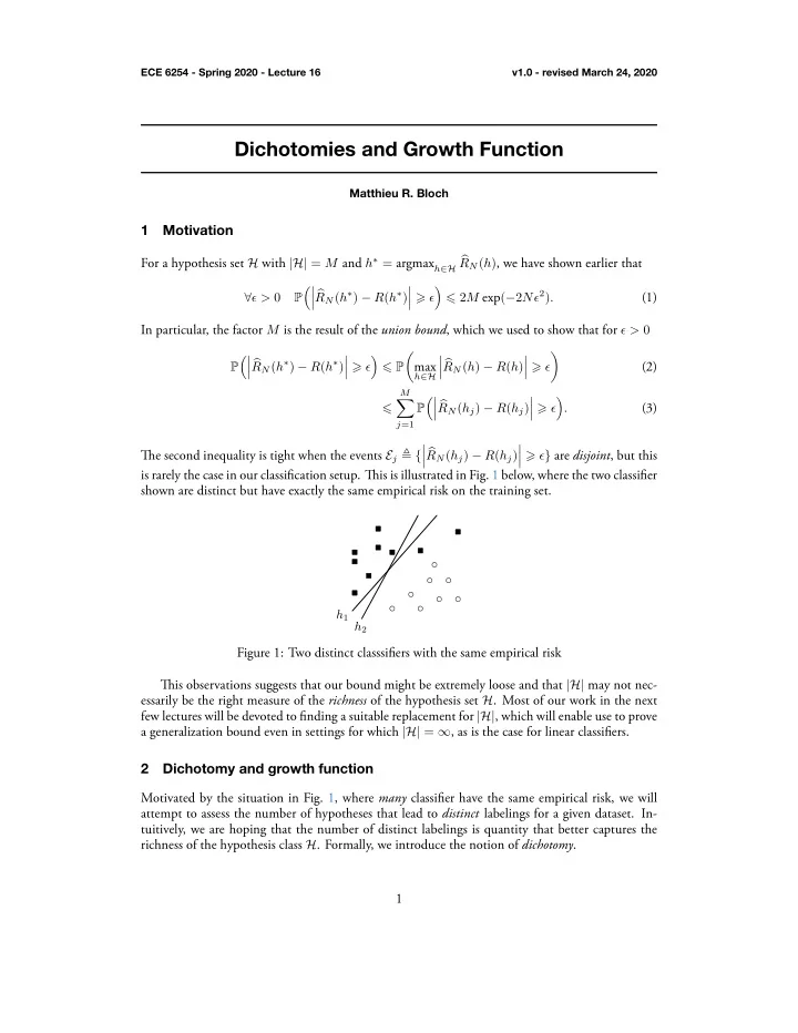
Definition 2.1 (Dichotomy). For a dataset D ≜ {xi}N

i=1 and set of hypotheses H, the set of dichotomies

generated by H on D is the set of labelings that can be generated by classfiers in H on the dataset, i.e., H({xi}N

i=1) ≜ {{h(xi)}N i=1 : h ∈ H}.

(4) Note that many sets {{h(xi)}N

i=1 for distinct h are actually identical because the labelings in-

duced on the dataset are identical. By definition, for our binary labeling problem,

• H({xi}N

i=1)

• ⩽

2N and in general

• H({xi}N

i=1)

• ≪ |H|. Unfortunately,
• H({xi}N

i=1)

• is not a particularly useful

quantity because it is not only potentially difficult to compute but also dependent on a specific

• dataset. Tiis motivates the definition of the growth function as follows.

Definition 2.2 (Growth function). For a set of hypotheses H, the growth function of H is mH(N) ≜ max

{xi}N

i=1

• H({xi}N

i=1)

• .

(5) Note that the growth function depends on the number of datapoints N but not on the exact datapoints {xi}N

i=1. Tie growth function measures the maximum number of dichotomies that H

can generate over all possible datasets, and by definition, it still holds that mH(N) ⩽ 2N. Example 2.3 (Positive rays). Consider a binary classification problem in R with the set of positive rays H ≜ {ha : R → {±1} : x → sign(x − a)|a ∈ R}. (6) As illustrated below, the threshold a defines a classifier such that all points to the left are assigned label −1 while all points to the right are assigned label +1.

h(x) = +1 h(x) = −1 x1 x2 xN xN−1 a

Although H = ∞, the number of dichotomies is still finite, and one can actually compute the growth function exactly. In general, this is challenging because we need to identify the worst case dataset that generates the highest number of dichotomies; here, this is only tractable because the situation is simple. Without losing generality, we can assume that all N points {xi}N

i=1 are distinct. Let us introduce

x0 ≜ −∞ and xN+1 ≜ ∞. For any i ⩾ 0, all classifiers ha with xi ⩽ a < xi+1 induce the same labeling. Consequently, the number of distinct labelings is at most N + 1 and mH(N) = N +

• 1. Interestingly, the growth function is growing polynomially in N, which is much slower than the

exponential growth 2N allowed by the upper bound. Example 2.4 (Positive intervals). Consider a binary classification in R with the set of positive intervals H ≜ {ha,b : R → {±1} : x → 1{x ∈ [a; b]} − 1{x / ∈ [a; b]} |a < b ∈ R}. (7) As illustrated below, the thresholds a < b define a classifier such that all points with [a; b] are assigned label +1 while all points outside are assigned label −1.

h(x) = +1 h(x) = −1 x1 x2 xN xN−1 a h(x) = −1 b

Again, this is a situation for which we can compute the growth function exactly. Without loss of generality, we assume that all N datapoints are distinct and we introduce x0 ≜ −∞ and xN+1 ≜ ∞. We need to be a bit more careful when counting dichotomies: 2

ECE 6254 - Spring 2020 - Lecture 16 v1.0 - revised March 24, 2020

• If x0 < a < b ⩽ x1, all classifiers hab induce an all-−1 labeling;
• for any 0 ⩽ i < j ⩽ N, all classifiers hab such that xi ⩽ a ⩽ xi+1 < xj ⩽ b ⩽ xj+1 induce

the same labelings;

• for any 0 ⩽ i ⩽ N, all classifiers hab such that xi ⩽ a < b < xi+1 induce again an all-−1

labeling. Consequently, the number of classifiers is 1 + N+1

2

and mH(N) = N 2

2 + N 2 + 1, which grows again

polynomially in N. 3