
1 Balls, Urns, and the Supreme Court
- Supreme Court case: Berghuis v. Smith
If a group is underrepresented in a jury pool, how do you tell?
- Article by Erin Miller – Friday, January 22, 2010
- Thanks to Josh Falk for pointing out this article
Justice Breyer [Stanford Alum] opened the questioning by invoking the binomial theorem. He hypothesized a scenario involving “an urn with a thousand balls, and sixty are red, and nine hundred forty are black, and then you select them at random… twelve at a time.” According to Justice Breyer and the binomial theorem, if the red balls were black jurors then “you would expect… something like a third to a half of juries would have at least one black person” on them.
- Justice Scalia’s rejoinder: “We don’t have any urns here.”
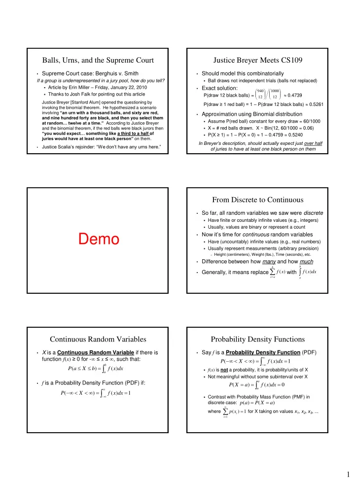
Justice Breyer Meets CS109
- Should model this combinatorially
- Ball draws not independent trials (balls not replaced)
- Exact solution:
P(draw 12 black balls) = 0.4739 P(draw ≥ 1 red ball) = 1 – P(draw 12 black balls) 0.5261
- Approximation using Binomial distribution
- Assume P(red ball) constant for every draw = 60/1000
- X = # red balls drawn. X ~ Bin(12, 60/1000 = 0.06)
- P(X ≥ 1) = 1 – P(X = 0) 1 – 0.4759 = 0.5240
In Breyer’s description, should actually expect just over half
- f juries to have at least one black person on them
12 1000 12 940
Demo
From Discrete to Continuous
- So far, all random variables we saw were discrete
- Have finite or countably infinite values (e.g., integers)
- Usually, values are binary or represent a count
- Now it’s time for continuous random variables
- Have (uncountably) infinite values (e.g., real numbers)
- Usually represent measurements (arbitrary precision)
- Height (centimeters), Weight (lbs.), Time (seconds), etc.
- Difference between how many and how much
- Generally, it means replace with
b a x
x f ) (
b a
dx x f ) (
Continuous Random Variables
- X is a Continuous Random Variable if there is
function f(x) ≥ 0 for - ≤ x ≤ , such that:
- f is a Probability Density Function (PDF) if:
b a
dx x f b X a P ) ( ) ( 1 ) ( ) (
dx x f X P
Probability Density Functions
- Say f is a Probability Density Function (PDF)
- f(x) is not a probability, it is probability/units of X
- Not meaningful without some subinterval over X
- Contrast with Probability Mass Function (PMF) in
discrete case: where for X taking on values x1, x2, x3, ...
) ( ) (
a a
dx x f a X P ) ( ) ( a X P a p
1 ) (
1
i i
x p
1 ) ( ) (
dx x f X P