Decision Making Under Uncertainty HW 3 out Group work for - PDF document

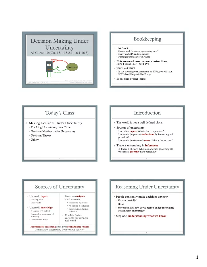
Bookkeeping Decision Making Under Uncertainty • HW 3 out • Group work for non-programming parts! AI C LASS 10 (C H . 15.1-15.2.1, 16.1-16.3) • Heavy on CSPs and probability • Forms groups today or in Piazza sensors • Note corrected error in turnin instructions: Parts I-III as PDF (not I-IV) ? environment • HW1 and HW2 agent • If you haven’t gotten comments on HW1, you will soon actuators • HW2 should be graded by Friday • Soon: form project teams! Material from Marie desJardin, Lise Getoor, Jean-Claude Latombe, Daphne Koller, and Paula Matuszek Cynthia Matuszek – CMSC 671 1 2 Today’s Class Introduction • The world is not a well-defined place. • Making Decisions Under Uncertainty • Tracking Uncertainty over Time • Sources of uncertainty • Decision Making under Uncertainty • Uncertain inputs : What’s the temperature? • Uncertain (imprecise) definitions : Is Trump a good • Decision Theory president? • Utility • Uncertain (unobserved) states : What’s the top card? • There is uncertainty in inferences • If I have a blistery, itchy rash and was gardening all weekend I probably have poison ivy 3 4 Sources of Uncertainty Reasoning Under Uncertainty • Uncertain outputs • Uncertain inputs • People constantly make decisions anyhow. • All uncertain: • Missing data • Very successfully! • Noisy data • Reasoning-by-default • How? • Abduction & induction • Uncertain knowledge • More formally: how do we reason under uncertainty • Incomplete deductive with inexact knowledge ? • >1 cause à >1 effect inference • Incomplete knowledge of • Result is derived • Step one: understanding what we know causality correctly but wrong in • Probabilistic effects real world Probabilistic reasoning only gives probabilistic results (summarizes uncertainty from various sources) 5 6 1

States and Observations P ART I: M ODELING U NCERTAINTY O VER T IME • Agents don’t have a continuous view of world • People don’t either! • We see things as a series of snapshots: • Observations , associated with time slices • t 1 , t 2 , t 3 , … • Each snapshot contains all variables, observed or not • X t = (unobserved) state variables at time t; observation at t is E t • This is world state at time t 7 8 Temporal Probabilistic Agent Uncertainty and Time • The world changes sensors • Examples: diabetes management, traffic monitoring • Tasks: track changes; predict changes ? environment • Basic idea: agent • For each time step, copy state and evidence variables • Model uncertainty in change over time (the Δ ) actuators • Incorporate new observations as they arrive t 1 , t 2 , t 3 , … 9 10 Uncertainty and Time States (more formally) • Basic idea: • Change is viewed as series of snapshots • Copy state and evidence variables for each time step • Time slices/timesteps • Model uncertainty in change over time • Each describing the state of the world at a particular time • Incorporate new observations as they arrive • So we also refer to these as states • X t = unobserved/unobservable state variables at time t: • Each time slice/timestep/state is represented as a BloodSugar t , StomachContents t set of random variables indexed by t : • E t = evidence variables at time t: 1. the set of unobservable state variables X t MeasuredBloodSugar t , PulseRate t , FoodEaten t 2. the set of observable evidence variables E t • Assuming discrete time steps 11 12 2

Observations (more formally) Transition and Sensor Models • So how do we model change over time? • Time slice (a set of random variables indexed by t ): This can get 1. the set of unobservable state variables X t • Transition model exponentially 2. the set of observable evidence variables E t • Models how the world changes over time large… • Specifies a probability distribution… • An observation is a set of observed variable • Over state variables at time t instantiations at some timestep P( X t | X 0:t-1 ) • Given values at previous times • Observation at time t : E t = e t • Sensor model • (for some values e t ) • Models how evidence (sensor data) gets its values • E.g.: BloodSugar t à MeasuredBloodSugar t • X a:b denotes the set of variables from X a to X b 13 14 Markov Assumption(s) Stationary Process • Markov Assumption : • Infinitely many possible values of t • X t depends on some finite (usually fixed) number of previous X i ’s • Does each timestep need a distribution? • That is, do we need a distribution of what the world looks like at • First-order Markov process : P( X t | X 0:t-1 ) = P( X t | X t-1 ) t 3 , given t 2 AND a distribution for t 16 given t 15 AND … • k th order: depends on previous k time steps • Assume stationary process : • Changes in the world state are governed by laws that do not themselves change over time • Sensor Markov assumption : P( E t | X 0:t , E 0:t-1 ) = P( E t | X t ) • Transition model P( X t | X t-1 ) and sensor model P( E t | X t ) are time-invariant, i.e., they are the same for all t • Agent’s observations depend only on actual current state of the world 15 16 Complete Joint Distribution Example Weather has a 30% chance • Given: R t-1 P(R t | R t-1 ) of changing and a 70% t 0.7 • Transition model: P( X t | X t-1 ) chance of staying the same. f 0.3 • Sensor model: P( E t | X t ) • Prior probability: P( X 0 ) Rain t-1 Rain t Rain t+1 • Then we can specify a complete joint distribution of a sequence of states: Umbrella t-1 Umbrella t Umbrella t+1 t ∏ P ( X 0 , X 1 ,..., X t , E 1 ,..., E t ) = P ( X 0 ) P ( X i | X i − 1 ) P ( E i | X i ) R t P(U t | R t ) t 0.9 i = 1 f 0.2 • What’s the joint probability of instantiations? 17 Fully worked out HMM for rain: www2.isye.gatech.edu/~yxie77/isye6416_17/Lecture6.pdf 3

Inference Tasks Examples • Filtering: What is the probability that it is raining today, • Filtering or monitoring: P( X t |e 1 ,…,e t ) : given all of the umbrella observations up through today? • Compute the current belief state, given all evidence to date • Prediction: What is the probability that it will rain the day • Prediction : P( X t+k |e 1 ,…,e t ) : after tomorrow, given all of the umbrella observations up • Compute the probability of a future state through today? • Smoothing : P( X k |e 1 ,…, et ) : • Smoothing: What is the probability that it rained yesterday, • Compute the probability of a past state (hindsight) given all of the umbrella observations through today? • Most likely explanation : arg max x1,..xt P(x 1 ,…,x t |e 1 ,…,e t ) • Most likely explanation: If the umbrella appeared the first three days but not on the fourth, what is the most likely • Given a sequence of observations, find the sequence of states that is weather sequence to produce these umbrella sightings? most likely to have generated those observations 19 20 Filtering Recursive Estimation • Maintain a current state estimate and update it 1. Project current state forward (t à t+1) • Instead of looking at all observed values in history 2. Update state using new evidence e t+1 • Also called state estimation • Given result of filtering up to time t , agent must P( X t+1 | e 1:t+1 ) as function of e t+1 and P( X t | e 1:t ): compute result at t+ 1 from new evidence e t+1 : P( X t +1 | e 1:t+1 ) = P( X t+1 | e 1:t , e t+1 ) P( X t+1 | e 1:t+1 ) = f ( e t+1 , P( X t | e 1:t )) … for some function f . 21 22 Recursive Estimation Recursive Estimation • One-step prediction by conditioning on current state X: • P( X t+1 | e 1:t+1 ) as a function of e t+1 and P( X t | e 1:t ): ∑ = α P ( e t + 1 | X t + 1 ) P ( X t + 1 | x t ) P ( x t | e 1: t ) P ( X t + 1 | e 1: t + 1 ) = P ( X t + 1 | e 1: t , e t + 1 ) dividing up evidence x t transition current = α P ( e t + 1 | X t + 1 , e 1: t ) P ( X t + 1 | e 1: t ) Bayes rule model state • …which is what we wanted! = α P ( e t + 1 | X t + 1 ) P ( X t + 1 | e 1: t ) sensor Markov assumption • P( e t+1 | X 1:t+1 ) updates with new evidence (from sensor) • So, think of P( X t | e 1:t ) as a “message” f 1:t+1 • Carried forward along the time steps • One-step prediction by conditioning on current state X: • Modified at every transition, updated at every new observation • This leads to a recursive definition: ∑ = α P ( e t + 1 | X t + 1 ) P ( X t + 1 | x t ) P ( x t | e 1: t ) f 1:t+1 = α FORWARD ( f 1:t , e t+1 ) x t 23 24 4