Curves and Splines Outline Hermite Splines Catmull-Rom Splines - - PowerPoint PPT Presentation

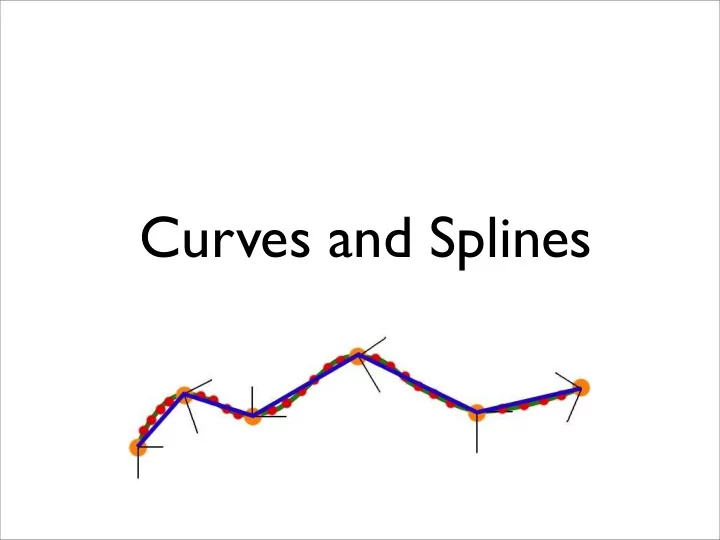
Curves and Splines

Outline

• Hermite Splines
• Catmull-Rom Splines
• Bezier Curves
• Higher Continuity: Natural and B-Splines
• Drawing Splines

3

Modeling Complex Shapes

• We want to build models of very complicated objects
• An equation for a sphere is possible, but how about an

equation for a telephone, or a face?

• Complexity is achieved

using simple pieces

– polygons, parametric curves and surfaces, or implicit curves and surfaces – This lecture: parametric curves

4

What Do We Need From Curves in Computer Graphics?

• Local control of shape (so that easy to build and

modify)

• Stability
• Smoothness and continuity
• Ability to evaluate derivatives
• Ease of rendering

Demo

Curve Usage Demo

5

Curve Representations

• Explicit: y = f(x)

– Easy to generate points – Must be a function: big limitation—vertical lines?

b mx y + =

x y

6

Curve Representations

• Explicit: y = f(x)

– Easy to generate points – Must be a function: big limitation—vertical lines?

b mx y + =

x y

• Implicit: f(x,y) = 0

+Easy to test if on the curve –Hard to generate points

2 2 2

= ! + r y x

x y

7

Curve Representations

• Explicit: y = f(x)

+ Easy to generate points – Must be a function: big limitation—vertical lines?

b mx y + =

x y

• Implicit: f(x,y) = 0

+Easy to test if on the curve –Hard to generate points

2 2 2

= ! + r y x

x y

• Parametric: (x,y) = ( f(u), g(u))

+Easy to generate points

) sin , (cos ) , ( u u y x =

u=0 u=" " " "/2 u= " " " "

8

Parameterization of a Curve

• Parameterization of a curve: how a change in u moves

you along a given curve in xyz space.

• There are an infinite number of parameterizations of a

given curve. Slow, fast, speed continuous or discontinuous, clockwise (CW) or CCW…

9

Polynomial Interpolation

• An n-th degree polynomial fits a curve to n+1 points

– called Lagrange Interpolation – result is a curve that is too wiggly, change to any control point affects entire curve (nonlocal) – this method is poor

• We usually want the curve to be as smooth as possible

– minimize the wiggles – high-degree polynomials are bad

Linear Interpolation

Chalkboard

Spline Interpolation

Spine Interpolation Demo

10

Splines: Piecewise Polynomials

• A spline is a piecewise polynomial - many low degree

polynomials are used to interpolate (pass through) the control points

• Cubic piecewise polynomials are the most common:

– piecewise definition gives local control

11

Piecewise Polynomials

• Spline: lots of little polynomials pieced together
• Want to make sure they fit together nicely

Continuous in position Continuous in position and tangent vector Continuous in position, tangent, and curvature

12

Splines

• Types of splines:

– Hermite Splines – Catmull-Rom Splines – Bezier Splines – Natural Cubic Splines – B-Splines – NURBS

7

Hermite Curves

• Cubic Hermite Splines

That is, we want a way to specify the end points and the slope at the end points!

Po P1 P2

13

Splines chalkboard

14

The Cubic Hermite Spline Equation

control matrix (what the user gets to pick) basis point that gets drawn

• Using some algebra, we obtain:

[ ]

! ! ! ! " # $ $ $ $ % & ! ! ! ! ! ! " # $ $ $ $ % & " " " " =

2 1 2 1 2 3

1 1 1 2 3 3 1 1 2 2 1 ) ( p p p p u u u u p

• This form typical for splines

– basis matrix and meaning of control matrix change with the spline type

15

The Cubic Hermite Spline Equation

control matrix (what the user gets to pick) basis point that gets drawn

• Using some algebra, we obtain:

[ ]

! ! ! ! " # $ $ $ $ % & ! ! ! ! ! ! " # $ $ $ $ % & " " " " =

2 1 2 1 2 3

1 1 1 2 3 3 1 1 2 2 1 ) ( p p p p u u u u p ! ! ! ! " # $ $ $ $ % & ! ! ! ! ! ! ! " # $ $ $ $ $ % & " + " + " + " =

2 1 2 1 2 3 2 3 2 3 2 3

2 3 2 1 3 2 ) ( p p p p u u u u u u u u u u p

4 Basis Functions T

16

Every cubic Hermite spline is a linear combination (blend)

• f these 4 functions

! ! ! ! " # $ $ $ $ % & ! ! ! ! ! ! ! " # $ $ $ $ $ % & " + " + " + " =

2 1 2 1 2 3 2 3 2 3 2 3

2 3 2 1 3 2 ) ( p p p p u u u u u u u u u u p

4 Basis Functions

Four Basis Functions for Hermite splines

T u

17

Piecing together Hermite Curves

• It's easy to make a multi-segment Hermite spline

– each piece is specified by a cubic Hermite curve – just specify the position and tangent at each “joint” – the pieces fit together with matched positions and first derivatives – gives C1 continuity

• The points that the curve has to pass through are called

knots or knot points

Outline

• Hermite Splines
• Catmull-Rom Splines
• Bezier Curves
• Higher Continuity: Natural and B-Splines
• Drawing Splines

Problem with Hermite Splines?

• Must explicitly specify derivatives at each

endpoint!

• How can we solve this?

8

Catmull-Rom Splines

• Use for the roller-coaster assignment
• With Hermite splines, the designer must specify all the

tangent vectors

• Catmull-Rom: an interpolating cubic spline with built-

in C1 continuity.

Po P1 P2 tangent at pi = s(pi+1 - pi-1)

18

Catmull-Rom Splines

• Use for the roller-coaster (next programming

assignment)

• With Hermite splines, the designer must arrange for

consecutive tangents to be collinear, to get C1

• continuity. This gets tedious.
• Catmull-Rom: an interpolating cubic spline with built-

in C1 continuity.

chalkboard

19

Catmull-Rom Spline Matrix

control vector CR basis

spline coefficients

[ ]

! ! ! ! " # $ $ $ $ % & ! ! ! ! " # $ $ $ $ % & ! ! ! ! ! ! ! =

4 3 2 1 2 3

1 2 3 3 2 2 2 1 ) ( p p p p s s s s s s s s s s u u u u p

• Derived similarly to Hermite
• Parameter s is typically set to s=1/2.

20

Catmull-Rom Spline Matrix

[ ] [

]

! ! ! ! " # $ $ $ $ % & ! ! ! ! " # $ $ $ $ % & ! ! ! ! ! ! ! =

4 4 4 3 3 3 2 2 2 1 1 1 2 3

1 2 3 3 2 2 2 1 z y x z y x z y x z y x s s s s s s s s s s u u u z y x

control vector CR basis

spline coefficients

9

Catmull-Rom Splines

• Use for the roller-coaster assignment
• With Hermite splines, the designer must specify all the

tangent vectors

• Catmull-Rom: an interpolating cubic spline with built-

in C1 continuity.

10

Catmull-Rom Spline Matrix

control vector CR basis

[ ]

! ! ! ! " # $ $ $ $ % & ! ! ! ! " # $ $ $ $ % & ! ! ! ! ! ! ! =

4 3 2 1 2 3

1 2 3 3 2 2 2 1 ) ( p p p p s s s s s s s s s s u u u u p

• Derived similarly to Hermite
• Parameter s is typically set to s=1/2.

11

Cubic Curves in 3D

• Three cubic polynomials, one for each coordinate

– x(u) = axu3+bxu2+cxu+dx – y(u) = ayu3+byu2+cyu+dy – z(u) = azu3+bzu2+czu+dz

• In matrix notation

[ ] [

]

! ! ! ! " # $ $ $ $ % & =

z y x z y x z y x z y x

d d d c c c b b b a a a u u u u z u y u x 1 ) ( ) ( ) (

2 3

12

Catmull-Rom Spline Matrix in 3D

[ ] [

]

! ! ! ! " # $ $ $ $ % & ! ! ! ! " # $ $ $ $ % & ! ! ! ! ! ! ! =

4 4 4 3 3 3 2 2 2 1 1 1 2 3

1 2 3 3 2 2 2 1 ) ( ) ( ) ( z y x z y x z y x z y x s s s s s s s s s s u u u u z u y u x

control vector CR basis

Outline

• Hermite Splines
• Catmull-Rom Splines
• Bezier Curves
• Higher Continuity: Natural and B-Splines
• Drawing Splines

Problem with Catmull-Rom Splines?

• No control of derivatives at endpoints!
• How can we solve this?
• We want something intuitive.

13

Bezier Curves*

• Another variant of the same game
• Instead of endpoints and tangents, four control points

– points P0 and P3 are on the curve: P(u=0) = P0, P(u=1) = P3 – points P1 and P2 are off the curve – P'(u=0) = 3(P1-P0), P'(u=1) = 3(P3 – P2)

• Convex Hull property

– curve contained within convex hull of control points

• Gives more control knobs (series of points) than Hermite
• Scale factor (3) is chosen to make “velocity” approximately constant

Bezier Spline Example

14

The Bezier Spline Matrix*

[ ] [

]

! ! ! ! " # $ $ $ $ % & ! ! ! ! " # $ $ $ $ % & ! ! ! ! =

4 4 4 3 3 3 2 2 2 1 1 1 2 3

1 3 3 3 6 3 1 3 3 1 1 z y x z y x z y x z y x u u u z y x

Bezier basis Bezier control vector

15

Bezier Blending Functions*

Also known as the order 4, degree 3 Bernstein polynomials Nonnegative, sum to 1 The entire curve lies inside the polyhedron bounded by the control points

Outline

• Hermite Splines
• Catmull-Rom Splines
• Bezier Curves
• Higher Continuity: Natural and B-Splines
• Drawing Splines

16

Piecewise Polynomials

• Spline: lots of little polynomials pieced together
• Want to make sure they fit together nicely

Continuous in position Continuous in position and tangent vector Continuous in position, tangent, and curvature

17

Splines with More Continuity?

• How could we get C2 continuity at control points?
• Possible answers:

– Use higher degree polynomials degree 4 = quartic, degree 5 = quintic, … but these get computationally expensive, and sometimes wiggly – Give up local control natural cubic splines A change to any control point affects the entire curve – Give up interpolation cubic B-splines Curve goes near, but not through, the control points

18

Comparison of Basic Cubic Splines

Type Local Control Continuity Interpolation Hermite YES C1 YES Bezier YES C1 YES Catmull-Rom YES C1 YES Natural NO C2 YES B-Splines YES C2 NO

• Summary

– Can’t get C2, interpolation and local control with cubics

19

Natural Cubic Splines*

• If you want 2nd derivatives at joints to match up, the

resulting curves are called natural cubic splines

• It’s a simple computation to solve for the cubics'
• coefficients. (See Numerical Recipes in C book for

code.)

• Finding all the right weights is a global calculation

(solve tridiagonal linear system)

20

B-Splines*

• Give up interpolation

– the curve passes near the control points – best generated with interactive placement (because it’s

hard to guess where the curve will go)

• Curve obeys the convex hull property
• C2 continuity and local control are good

compensation for loss of interpolation

21

B-Spline Basis*

• We always need 3 more control points than spline

pieces

! ! ! ! " # $ $ $ $ % & = ! ! ! ! " # $ $ $ $ % & ! ! ! ! =

! ! ! i i i i Bs Bs

P P P P G M

i

1 2 3

1 4 1 3 3 3 6 3 1 3 3 1 6 1

Outline

• Hermite Splines
• Catmull-Rom Splines
• Bezier Curves
• Higher Continuity: Natural and B-Splines
• Drawing Splines

22

How to Draw Spline Curves

• Basis matrix eqn. allows same code to draw any spline type
• Method 1: brute force

– Calculate the coefficients – For each cubic segment, vary u from 0 to 1 (fixed step size) – Plug in u value, matrix multiply to compute position on curve – Draw line segment from last position to current position

[ ] [

]

! ! ! ! " # $ $ $ $ % & ! ! ! ! " # $ $ $ $ % & ! ! ! ! ! ! ! =

4 4 4 3 3 3 2 2 2 1 1 1 2 3

1 2 3 3 2 2 2 1 z y x z y x z y x z y x s s s s s s s s s s u u u z y x

control vector CR basis

23

How to Draw Spline Curves

• What’s wrong with this approach?

–Draws in even steps of u –Even steps of u ! ! ! ! even steps of x –Line length will vary over the curve –Want to bound line length

»too long: curve looks jagged »too short: curve is slow to draw

24

Drawing Splines, 2

• Method 2: recursive subdivision - vary step size to draw short lines

Subdivide(u0,u1,maxlinelength) umid = (u0 + u1)/2 x0 = P(u0) x1 = P(u1) if |x1 - x0| > maxlinelength Subdivide(u0,umid,maxlinelength) Subdivide(umid,u1,maxlinelength) else drawline(x0,x1)

• Variant on Method 2 - subdivide based on curvature

– replace condition in “if” statement with straightness criterion – draws fewer lines in flatter regions of the curve

25

In Summary...

• Summary:

– piecewise cubic is generally sufficient – define conditions on the curves and their continuity

• Things to know:

– basic curve properties (what are the conditions, controls, and properties for each spline type) – generic matrix formula for uniform cubic splines x(u) = uBG – given definition derive a basis matrix