cse 571
play

CSE-571 So far, we discussed the Kalman filter: Gaussian, - PowerPoint PPT Presentation

Motivation CSE-571 So far, we discussed the Kalman filter: Gaussian, linearization problems Robotics Particle filters are a way to efficiently represent non-Gaussian distributions Bayes Filter Implementations Basic principle Set


  1. Motivation CSE-571 § So far, we discussed the § Kalman filter: Gaussian, linearization problems Robotics § Particle filters are a way to efficiently represent non-Gaussian distributions Bayes Filter Implementations § Basic principle § Set of state hypotheses ( “ particles ” ) Particle filters § Survival-of-the-fittest 2 
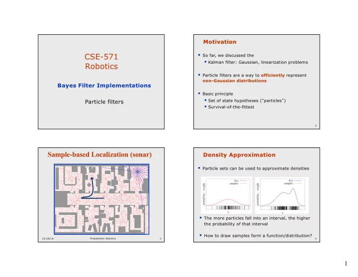
Sample-based Localization (sonar) Density Approximation § Particle sets can be used to approximate densities § The more particles fall into an interval, the higher the probability of that interval § How to draw samples form a function/distribution? 10/18/16 Probabilistic Robotics 3 4 1

  2. Rejection Sampling Importance Sampling Principle § Let us assume that f(x)<= 1 for all x § We can even use a different distribution g to § Sample x from a uniform distribution generate samples from f § By introducing an importance weight w , we can § Sample c from [0,1] account for the “ differences between g and f ” § if f(x) > c keep the sample § w = f / g otherwise reject the sampe § f is often called target § g is often called f(x’) c proposal c’ OK f(x) x x ’ 5 6 Importance Sampling with Resampling: Distributions Landmark Detection Example Wanted: samples distributed according to p(x| z 1 , z 2 , z 3 ) 2

  3. Importance Sampling with This is Easy! Resampling We can draw samples from p(x|z l ) by adding Õ p ( z | x ) p ( x ) noise to the detection parameters. k = k Target distributi on f : p ( x | z , z ,..., z ) 1 2 n p ( z , z ,..., z ) 1 2 n Sampling distribution g: p ( x | z l ) = p ( z l | x ) p ( x ) p ( z l ) Õ p ( z ) p ( z | x ) l k f p ( x | z , z ,..., z ) = = Importance weights w : 1 2 n k ¹ l g p ( x | z ) p ( z , z ,..., z ) l 1 2 n Importance Sampling with Resampling Resampling • Given : Set S of weighted samples. • Wanted : Random sample, where the probability of drawing x i is given by w i . • Typically done n times with replacement to generate new sample set S ’ . Weighted samples After resampling 3

  4. Resampling Algorithm Resampling 1. Algorithm systematic_resampling ( S,n ): w 1 w 1 w n w n w 2 2. w 2 = Æ = 1 S ' , c w W n-1 W n-1 1 3. For = ! Generate cdf i 2 n w 3 w 3 = + i 4. c c w i i - 1 - 1 = 5. u ~ U [ 0 , n ], i 1 Initialize threshold 1 = 6. For j 1 ! n Draw samples … u > 7. While ( ) c Skip until next threshold reached j i = i + 8. i 1 { } • Stochastic universal sampling = È < i - 1 > 9. S ' S ' x , n Insert • Roulette wheel • Systematic resampling = + - 1 10. u u n Increment threshold j j • Binary search, n log n • Linear time complexity • Easy to implement, low variance 11. Return S ’ Also called stochastic universal sampling Sensor Information: Importance Sampling Particle Filters - ¬ a Bel ( x ) p ( z | x ) Bel ( x ) a - p ( z | x ) Bel ( x ) ¬ = a w p ( z | x ) - Bel ( x ) 4

  5. Sensor Information: Importance Sampling Robot Motion - ¬ a Bel ( x ) p ( z | x ) Bel ( x ) ò - ¬ Bel ( x ) p ( x | u x ' ) Bel ( x ' ) d x ' , a - p ( z | x ) Bel ( x ) ¬ = a w p ( z | x ) - Bel ( x ) Robot Motion Particle Filter Algorithm ò - ¬ Bel ( x ) p ( x | u x ' ) Bel ( x ' ) d x ' , 1. Algorithm particle_filter ( S t-1 , u t-1 z t ): 2. = Æ h = S , 0 t 3. For = Generate new samples i 1 ! n 4. Sample index j(i) from the discrete distribution given by w t-1 5. Sample from using and i p ( x | x , u ) j ( i ) u x x - - - - t t t 1 t 1 t 1 t 1 6. w = i i Compute importance weight p ( z | x ) t t t 7. h = h + i Update normalization factor w t 8. = È < > Insert S S { x i , w i } t t t t 9. For = i 1 ! n 10. w = i i h Normalize weights w / t t 5

  6. Motion Model Reminder Particle Filter Algorithm ò = h Bel ( x ) p ( z | x ) p ( x | x , u ) Bel ( x ) dx - - - - t t t t t 1 t 1 t 1 t 1 draw x it - 1 from Bel (x t - 1 ) draw x it from p ( x t | x it - 1 , u t - 1 ) Importance factor for x it : target distributi on i = w t proposal distributi on h p ( z | x ) p ( x | x , u ) Bel ( x ) = - - - t t t t 1 t 1 t 1 Start p ( x | x , u ) Bel ( x ) t t - 1 t - 1 t - 1 µ p ( z | x ) t t Proximity Sensor Model Reminder Sonar sensor Laser sensor 24 6

  7. 25 26 27 28 7

  8. 29 30 31 32 8

  9. 33 34 35 36 9

  10. 37 38 39 40 10

  11. Using Ceiling Maps for Localization 41 [Dellaert et al. 99] Vision-based Localization Under a Light Measurement z: P(z|x) : P(z|x) z h(x) 11

  12. Next to a Light Elsewhere Measurement z: P(z|x) : Measurement z: P(z|x) : Recovery from Failure Global Localization Using Vision 12

  13. Adaptive Sampling Localization for AIBO robots KLD-Sampling Sonar KLD-Sampling Laser Adapt number of particles on the fly based on statistical approximation measure 13

  14. Particle Filter Projection Density Extraction Sampling Variance CSE-571 Robotics Bayes Filter Implementations Discrete filters SA-1 14

  15. Discrete Bayes Filter Algorithm Piecewise Algorithm Discrete_Bayes_filter ( Bel(x),d ): 1. Constant 2. h = 0 3. If d is a perceptual data item z then 4. For all x do = Bel ' ( x ) P ( z | x ) Bel ( x ) 5. h = h + Bel ' x ( ) 6. 7. For all x do = h - 1 8. Bel ' ( x ) Bel ' ( x ) 9. Else if d is an action data item u then 10. For all x do å = 11. Bel ' ( x ) P ( x | u , x ' ) Bel ( x ' ) x ' 12. Return Bel ’ (x) 10/18/16 CSE-571 - Probabilistic Robotics 57 10/18/16 CSE-571 - Probabilistic Robotics 58 Piecewise Constant Grid-based Localization Representation =< q > Bel ( x x , y , ) t 10/18/16 CSE-571 - Probabilistic Robotics 59 10/18/16 CSE-571 - Probabilistic Robotics 60 15

  16. Sonars and Tree-based Representation Occupancy Grid Map Idea : Represent density using a variant of Octrees 10/18/16 CSE-571 - Probabilistic Robotics 61 10/18/16 CSE-571 - Probabilistic Robotics 62 Localization Algorithms - Comparison Tree-based Representations Kalman Multi- Topological Grid-based Particle filter hypothesis filter maps (fixed/variable) tracking • Efficient in space and time Sensors Gaussian Gaussian Features Non-Gaussian Non- • Multi-resolution Gaussian Posterior Gaussian Multi-modal Piecewise Piecewise Samples constant constant Efficiency (memory) ++ ++ ++ -/o +/++ Efficiency (time) ++ ++ ++ o/+ +/++ Implementation + o + +/o ++ Accuracy ++ ++ - +/++ ++ Robustness - + + ++ +/++ Global No Yes Yes Yes Yes localization 10/18/16 CSE-571 - Probabilistic Robotics 63 16

Download Presentation
Download Policy: The content available on the website is offered to you 'AS IS' for your personal information and use only. It cannot be commercialized, licensed, or distributed on other websites without prior consent from the author. To download a presentation, simply click this link. If you encounter any difficulties during the download process, it's possible that the publisher has removed the file from their server.

Recommend


More recommend