
SLIDE 1
1
SA-1
CSE-571 Robotics
Probabilistic Sensor Models Beam-based Scan-based Landmarks
1
CSE-571 - Robotics 4/15/20 2
Sensors for Mobile Robots
- Contact sensors: Bumpers
- Internal sensors
- Accelerometers (spring-mounted masses)
- Gyroscopes (spinning mass, laser light)
- Compasses, inclinometers (earth magnetic field, gravity)
- Proximity sensors
- Sonar (time of flight)
- Radar (phase and frequency)
- Laser range-finders (triangulation, tof, phase)
- Infrared (intensity)
- Visual sensors: Cameras, depth cameras
- Satellite-based sensors: GPS
2
CSE-571 - Robotics 4/15/20 3
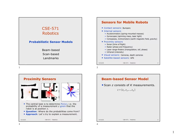
Proximity Sensors
- The central task is to determine P(z|x), i.e. the
probability of a measurement z given that the robot is at position x.
- Question: Where do the probabilities come from?
- Approach: Let’s try to explain a measurement.
3
CSE-571 - Robotics 4/15/20 4
Beam-based Sensor Model
- Scan z consists of K measurements.
} ,..., , {
2 1 K