CS4811 Neural Network Training Example Consider the following - PDF document

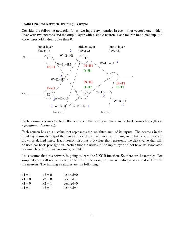
CS4811 Neural Network Training Example Consider the following network. It has two inputs (two entries in each input vector), one hidden layer with two neurons and the output layer with a single neuron. Each neuron has a bias input to allow threshold values other than 0. input layer hidden layer output layer (layer 1) 2 (layer 2) (layer 3) W−I1−H1 x1 I1 H1 3 W−H1−T1 W−I1−H2 IN−H1 IN−I1 1 D−H1 −2 T1 W−I2−H1 IN−H2 IN−T1 D−H2 D−T1 IN−I2 W−H2−T2 x2 H2 I2 −2 W−I2−H2 3 W−B−T1 −1 0 W−B−H1 W−B−H2 −1 bias = 1 bias = 1 Each neuron is connected to all the neurons in the next layer, there are no back connections (this is a feedforward network ). Each neuron has an IN value that represents the weighted sum of its inputs. The neurons in the input layer simply output their input, they don’t have weights coming in. That is why they are drawn as dashed lines. Each neuron also has a D value that represents the delta value that will be used for back propagation. Notice that the nodes in the input layer do not have D s associated because they don’t have incoming weights. Let’s assume that this network is going to learn the NXOR function. So there are 4 examples. For simplicity we will not be showing the bias in the examples, we will always assume it is 1 for all the neurons. The training examples are the following: x1 = 1 x2 = 0 desired=0 x1 = 0 x2 = 0 desired=1 x1 = 0 x2 = 1 desired=0 x1 = 1 x2 = 1 desired=1 1

We will first initialize the weights to random values: W-I1-H1 = 2 W-I1-H2 = 1 W-I2-H1 = -2 W-I2-H2 = 3 W-B-H1 = 0 W-B-H2 = -1 W-H1-T1 = 3 W-H2-T1 = -2 W-B-T1 = -1 We will now do a complete pass with the first training example x1 = 1, x2 = 0 and the de- sired output is 0 . We first compute the output of all the neurons. For that, we will use the sigmoid function rather than the threshold function because it is differentiable. If f is the sigmoid function, then its differential is f (1 − f ) . The sigmoid function is defined as follows: 1 1 + e − x The input layer simply transfers to the input to the output. These neurons don’t have a bias input. IN-I1 = a I 1 = x 1 IN-I2 = a I 2 = x 2 The other neurons compute a weighted sum of their inputs and evaluate the activation value. This corresponds to the feed forward loop: j W j,i a j IN-H1 = � = x 1 × W-I1-H1 + x 2 × W-I2-H1 + bias × W-B-H1 = 1 × 2 + 0 × − 2 + 1 × 0 = 2 A-H1 = sigmoid ( IN-H1 ) = sigmoid (2) = 0.880797. Similarly, IN-H2 = 0, A-H2 = 0.5, and IN-T1 = 0.642391, and A-T1 = 0.655294. 2

Next we will compute the delta ( ∆ ) values. Remember that g ′ for sigmoid is g (1 − g ) . We start with the output layer using the following lines from the algorithm: for each node j in the output layer do // Compute the error at the output. ∆[ j ] ← g ′ ( in j ) × ( y j − a j ) D-T1 = A-T1 × (1- A-T1 ) × (desired - A-T1 ) = -0.148020. We continue with the two nodes in the hidden layer using the following lines from the algorithm: /* Propagate the deltas backward from output layer to input layer */ for l = L − 1 to 1 do for each node i in layer l do ∆[ i ] ← g ′ ( in i ) � j w i,j ∆[ j ] // “Blame” a node as much as its weight. D-H1 = A-H1 × (1 - A-H1 ) × W-H1-T1 × D-T1 = -0.0446624. D-H2 = A-H2 × (1 - A-H2 ) × W-H2-T1 × D-T1 = 0.074010. 3

Now we have all the values we need, we will perform backpropagation and update the weights. We will use a learning constant c of 1. If another value is used, it multiplies the term after the sum. The following are the corresponding lines from the algorithm: /* Update every weight in network using deltas. */ for each weight w i,j in network do w i,j ← w i,j + α × a i × ∆[ j ] // Adjust the weights. There are 3 sets of 3 weights. Each set is for a non-input neuron: W-H1-T1 = W-H1-T1 + c × A-H1 × D-T1 = 3 + 1 × 0.880797 × -0.148020 = 2.869624. W-H2-T1 = W-H2-T1 + c × A-H2 × D-T1 = -2.074010. W-B-T1 = W-B-T1 + c × 1 × D-T1 = -1.148020. W-I1-H1 = W-I1-H1 + c × x 1 × D-H1 = 1.953376. W-I2-H1 = W-I2-H1 + c × x 2 × D-H1 = -2.000000. W-B-H1 = W-B-H1 + c × 1 × D-H1 = -0.046624. W-I1-H2 = W-I1-H2 + c × x 1 × D-H2 = 1.074010. W-I2-H2 = W-I2-H2 + c × x 2 × D-H2 = 3.000000. W-B-H2 = W-B-H2 + c × 1 × D-H2 = -0.925990. The above are the weights after the first example is processed. A similar procedure is followed several times for each example until the network converges or an iteration limit is reached. To test the network, we go back to using the threshold function (not the sigmoid). 4