
SLIDE 1
CS440/ECE448 Lecture 18: Hidden Markov Models
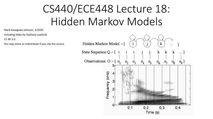
Mark Hasegawa-Johnson, 3/2020 Including slides by Svetlana Lazebnik CC-BY 3.0 You may remix or redistribute if you cite the source.
CS440/ECE448 Lecture 18: Hidden Markov Models Mark - - PowerPoint PPT Presentation
CS440/ECE448 Lecture 18: Hidden Markov Models Mark Hasegawa-Johnson, 3/2020 Including slides by Svetlana Lazebnik CC-BY 3.0 You may remix or redistribute if you cite the source. Probabilistic reasoning over time So far, weve mostly
Mark Hasegawa-Johnson, 3/2020 Including slides by Svetlana Lazebnik CC-BY 3.0 You may remix or redistribute if you cite the source.
problem instance
tracking, speech recognition, machine translation,
X0 E1 X1 Et-1 Xt-1 Et Xt
E2 X2
states given the state in the previous time step
P(Xt | X0:t-1) = P(Xt | Xt-1)
P(Et | X0:t, E1:t-1) = P(Et | Xt) X0 E1 X1 Et-1 Xt-1 Et Xt
E2 X2
Characters from the novel Hammered by Elizabeth Bear, Scenario from chapter 15 of Russell & Norvig
state
Characters from the novel Hammered by Elizabeth Bear, Scenario from chapter 15 of Russell & Norvig
state
Transition model Observation model
Characters from the novel Hammered by Elizabeth Bear, Scenario from chapter 15 of Russell & Norvig
state
Transition model Observation model
R=T R=F 0.7 0.7 0.3 0.3 U=T: 0.9 U=F: 0.1 U=T: 0.2 U=F: 0.8
Ut = T Ut = F Rt = T 0.9 0.1 Rt = F 0.2 0.8
Observation probabilities
Rt = T Rt = F Rt-1 = T 0.7 0.3 Rt-1 = F 0.3 0.7
Transition probabilities
R=T R=F 0.7 0.7 0.3 0.3
(continuous valued)
(so, tens of thousands)
(continuous)
Source: Tamara Berg
Acoustic wave form Sampled at 16KHz, quantized to 8-12 bits Time Frequency FFT of one frame (10ms) is the HMM observation,
Observation = compressed version of the log magnitude FFT, from one 10ms frame
Fast Fourier Transform (FFT), once per 10ms, computes a ”picture” whose axes are time and frequency
specific word, coded using the international phonetic alphabet:
SIL
0.95 0.05
0.1 0.5 SIL 1.0 0.2 0.8
0.5 0.9 Finite State Machine model of the word “Beth”
X0 E1 X1 Et-1 Xt-1 Et Xt
E2 X2
=
t i i i i i :t :t
1 1 1
the evidence so far, E1:t ? (example: is it currently raining?) X0 E1 X1 Et-1 Xt-1 Et Xt
Ek Xk Query variable Evidence variables
the evidence so far, E1:t ?
the entire observation sequence E1:t? (example: did it rain on Sunday?) X0 E1 X1 Et-1 Xt-1 Et
Ek Xk
Xt Query variable
the evidence so far, E1:t ?
the entire observation sequence E1:t?
sequence E1:t (example: is Richard using the right model?) X0 E1 X1 Et-1 Xt-1 Et
Ek Xk
Xt Query: Is this the right model for these data?
the evidence so far, E1:t
the entire observation sequence E1:t?
sequence E1:t
day?) X0 E1 X1 Et-1 Xt-1 Et
Ek Xk
Xt Query variables: all of them
given all the evidence so far, E1:t
given the entire observation sequence E1:t?
sequence E1:t
parameters (transition and emission probabilities)
state
Transition model
'!,'"
R0 U1 R1 U2 R2
Ut = T Ut = F Rt = T 0.9 0.1 Rt = F 0.2 0.8
Observation probabilities
Rt = T Rt = F Rt-1 = T 0.7 0.3 Rt-1 = F 0.3 0.7
Transition probabilities
'#,'!
R0 U1 R1 Ut-1 Rt-1 Ut Rt
U2 R2
state
Transition model
1. Select: To represent the relationship among 𝑄 𝑆#|¬𝑉", 𝑉# ? …we also need knowledge of 𝑆! and 𝑆".
probability, 𝑄 𝑆! .
statement! Therefore we are justified in making any reasonable assumption, and clearly stating our assumption. Let’s assume 𝑄 𝑆! = 0.5 R0 U1 R1 U2 R2
Ut = T Ut = F Rt = T 0.9 0.1 Rt = F 0.2 0.8
Observation probabilities
Rt = T Rt = F Rt-1 = T 0.7 0.3 Rt-1 = F 0.3 0.7
Transition probabilities
state
Transition model
𝑄 𝑆!, 𝑆", 𝑆#, 𝑉",𝑉# = 𝑄 𝑆! 𝑄 𝑆"|𝑆! 𝑄 𝑉"|𝑆" … 𝑄 𝑉#|𝑆#
R0 U1 R1 U2 R2
Ut = T Ut = F Rt = T 0.9 0.1 Rt = F 0.2 0.8
Observation probabilities
Rt = T Rt = F Rt-1 = T 0.7 0.3 Rt-1 = F 0.3 0.7
Transition probabilities
¬𝑺𝟑¬𝑽𝟑¬𝑺𝟑𝑽𝟑 𝑺𝟑¬𝑽𝟑 𝑺𝟑𝑽𝟑 ¬𝑺𝟏¬𝑺𝟐¬𝑽𝟐 0.1568 0.0392 0.0084 0.0756 ¬𝑺𝟏¬𝑺𝟐𝑽𝟐 0.0392 0.0098 0.0021 0.0189 ¬𝑺𝟏𝑺𝟐¬𝑽𝟐 0.0036 0.0009 0.0011 0.0095 ¬𝑺𝟏𝑺𝟐𝑽𝟐 0.0324 0.0081 0.0095 0.0851 𝑺𝟏¬𝑺𝟐¬𝑽𝟐 0.0672 0.0168 0.0036 0.0324 𝑺𝟏¬𝑺𝟐𝑽𝟐 0.0168 0.0042 0.009 0.0081 𝑺𝟏𝑺𝟐¬𝑽𝟐 0.0084 0.0021 0.0025 0.0221 𝑺𝟏𝑺𝟐𝑽𝟐 0.0756 0.0189 0.0221 0.1985
state
Transition model
3. Add: 𝑄 𝑆#, 𝑉",𝑉# = .
'!,'"
𝑄 𝑆!, 𝑆", 𝑆#, 𝑉",𝑉# R0 U1 R1 U2 R2
Ut = T Ut = F Rt = T 0.9 0.1 Rt = F 0.2 0.8
Observation probabilities
Rt = T Rt = F Rt-1 = T 0.7 0.3 Rt-1 = F 0.3 0.7
Transition probabilities
¬𝑽𝟐¬𝑽𝟑¬𝑽𝟐𝑽𝟑 𝑽𝟐¬𝑽𝟑 𝑽𝟐𝑽𝟑 ¬𝑺𝟑 0.236 0.059 0.164 0.041 𝑺𝟑 0.0155 0.1395 0.0345 0.3105
state
Transition model
R0 U1 R1 U2 R2
Ut = T Ut = F Rt = T 0.9 0.1 Rt = F 0.2 0.8
Observation probabilities
Rt = T Rt = F Rt-1 = T 0.7 0.3 Rt-1 = F 0.3 0.7
Transition probabilities
¬𝑽𝟐¬𝑽𝟑¬𝑽𝟐𝑽𝟑 𝑽𝟐¬𝑽𝟑 𝑽𝟐𝑽𝟑 ¬𝑺𝟑 0.94 0.30 0.83 0.12 𝑺𝟑 0.06 0.70 0.17 0.88