CS 598 RM : Algorithmic game theory Lecture 1 Two-player games For - - PDF document

CS 598 RM : Algorithmic game theory Lecture 1

Two-player games

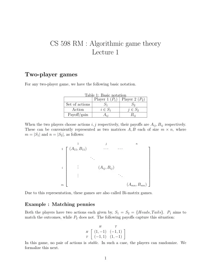
For any two-player game, we have the following basic notation. Table 1: Basic notation Player 1 (P1) Player 2 (P2) Set of actions S1 S2 Action i ∈ S1 j ∈ S2 Payoff/gain Aij Bij When the two players choose actions i, j respectively, their payoffs are Aij, Bij respectively. These can be conveniently represented as two matrices A, B each of size m × n, where m = |S1| and n = |S2|, as follows:            

1 j n 1

(A11, B11) · · · · · · ...

i

. . . (Aij, Bij) . . . ...

m

(Amn, Bmn)             Due to this representation, these games are also called Bi-matrix games.

Example : Matching pennies

Both the players have two actions each given by, S1 = S2 = {Heads, Tails}. P1 aims to match the outcomes, while P2 does not. The following payoffs capture this situation:

• H

T H

(1, −1) (−1, 1)

T

(−1, 1) (1, −1)

• In this game, no pair of actions is stable. In such a case, the players can randomize. We

formalize this next. 1

More notation and fundamentals

The randomization between possible actions, is achieved by what is called a mixed strategy. We denote the set of mixed strategies for P1 and P2, by ∆1 and ∆2 respectively, given by, ∆1 = {x = (x1, x2, . . . , x|S1|) | xi ≥ 0 ∀i ∈ S1, and

• i∈S1

xi = 1} and, ∆2 = {y = (y1, y2, . . . , y|S2|) | yj ≥ 0 ∀j ∈ S2, and

• j∈S2

yj = 1} When the two players play strategies x ∈ ∆1 and y ∈ ∆2 respectively, the expected payoff

• f P1 is given by

i∈S1 j∈S2

Aijxiyj = xTAy, and similarly, that of P2 is xTBy. Thus, P1 tries to maximize xTAy, and P2 tries to maximize xTBy. Definition (Nash equilibrium). A strategy profile (x′, y′) is a Nash Equilibrium (NE) iff x′ ∈ argmax

x∈∆1

xTAy′ and y′ ∈ argmax

y∈∆2

x′TBy Having defined the NE, one would like to answer the following questions:

• How to check if a given strategy profile is a NE?
• Does a NE exist in a given game? In every game?
• How to compute a NE?

Theorem (Nash ’51). Every n-player game has a NE (n ∈ N).

Characterization of NE

Fix y for P2. Then, P1 gets a payoff of (Ay)i from action i ∈ S1. Thus, the maximum possible from any action is max

i∈S1 (Ay)i = (say) v. Hence, playing x gives P1 a payoff of

xTAy =

• i∈S1

xi(Ay)i = convex combination of (Ay)i’s ∴ xTAy ≤ v & xTAy = v iff (∀i ∈ S1, (xi > 0 ⇒ (Ay)i = v)) A similar analysis works for P2 as well. Fixing P1’s strategy to x, P2 gets a payoff of (xTB)j from action j ∈ S2. Letting w = max

j∈S2 (xTB)j, we can deduce,

∀y ∈ ∆2, xTBy ≤ w & xTBy = w iff (∀j ∈ S2, (yj > 0 ⇒ (xTB)j = w)) We summarize this analysis as the following theorem characterizing Nash Equilibria: 2

Theorem 1. (x, y) is a NE iff ∀i ∈ S1 : xi > 0 ⇒ (Ay)i = v and, ∀j ∈ S2 : yj > 0 ⇒ (xTB)j = w where, v = max

i∈S1 (Ay)i

& w = max

j∈S2 (xTB)j

This theorem allows us to easily check if a strategy profile is NE.

Zero-sum games

In these games, we have, Bij = −Aij ∀i ∈ S1, ∀j ∈ S2, i.e., simply B = −A Hence, these games are described by just one matrix A. P1 tries to maximize its payoff, and thus, maximize xTAy. Similarly, P2 tries to maximize xT(−A)y, and thus, minimize xTAy. Hence, P1 is called the maximizer and P2 is called the minimizer. Minimax play in zero-sum games Suppose both the players play pessimistically. To elaborate, P1 assumes that P2 can find

• ut its strategy x, ahead of time and play y accordingly to achieve its goal of minimization
• f xTAy. P2 has a similar approach in choosing its strategy. Suppose they decide x∗, y∗ as

their strategies respectively, by playing pessimistically as described. Then, it must mean, x∗ ∈ argmax

x∈∆1

• min

y∈∆2 xTAy

• &

y∗ ∈ argmin

y∈∆2

• max

x∈∆1 xTAy

• Now, let π1 denote P1’s guaranteed payoff, that is, the minimum worst-case payoff it can

ensure - precisely as demonstrated in the pessimistic approach mentioned above. That is, π1 = max

x∈∆1

• min

y∈∆2 xTAy

• (1)

= min

y∈∆2 x∗TAy

(2) Similarly, let π2 be P2’s guaranteed payoff, that is, π2 = min

y∈∆2

• max

x∈∆1 xTAy

• (3)

= max

x∈∆1 xTAy∗

(4) We now show a remarkable result. 3

Theorem 2. For x∗, y∗, π1, π2 as defined above, the following hold.

• 1. π1 = π2 = x∗TAy∗
• 2. If (x′, y′) is a NE, then, x′TAy′ = x∗TAy∗
• 3. (x∗, y∗) is a NE.
• Proof. Using the definition of π1 as in (2), it follows that, π1 ≤ x∗TAy∗.

Similarly, using the definition of π2 in (4), it follows that, π2 ≥ x∗TAy∗. Combining the two, we get, π1 ≤ x∗TAy∗ ≤ π2 (5) Further, for a NE (x′, y′), by definition of NE, we have, x′TAy′ = max

x∈∆1 xTAy′

(6) x′TAy′ = min

y∈∆2 x′TAy

(7) From (7) and (1), we get, π1 ≥ x′TAy′. Similarly, from (6) and (3), we get, π2 ≤ x′TAy′. Combining the two, we get, π2 ≤ x′TAy′ ≤ π1 (8) (5) and (8) together prove the first two parts of the theorem. Having proven π2 = x∗TAy∗, and again from the definition of π2 in (2), it follows that x∗ ∈ argmax

x∈∆1

xTAy∗. Similarly, we can get y∗ ∈ argmin

y∈∆2

x∗TAy. Hence, (x∗, y∗) is a NE by definition, proving part 3 of the theorem. Linear Programming Formulation (in zero-sum games) Suppose the players are playing to optimize their worst-case payoffs as in the previous section. From P2’s perspective, fixing its strategy to y ∈ ∆2, P1’s best payoff is max

i∈S1 (Ay)i = (say) vy.

Hence, to minimize this, P2 wants to solve for min

y∈∆2 vy - equivalently, this linear program LP:

min v s.t. v ≥ (Ay)i ∀i ∈ S1, (1)

• j∈S2

yj = 1, (2) yj ≥ 0 ∀j ∈ S2 (3) 4

The constraints in (2) and (3) ensure that y ∈ ∆2. Letting the dual variables corresponding to the inequalities in (1) be xi’s and the dual variable corresponding to (2) be w, the dual DLP of the linear program above, can be written as, max w s.t. w ≤ (xTA)j ∀j ∈ S2, (4)

• i∈S1

xi = 1, (5) xi ≥ 0 ∀i ∈ S1 (6) Then, it’s easy to see that DLP is equivalent to solving for max

x∈∆1 wx, where, wx = min j∈S2 (xTA)j,

and the constraints in (5) and (6) ensure that x ∈ ∆1. Thus, this is precisely what P1 wants to do to maximize its worst-case payoff. Consequently, we have the following theorem: Theorem 3. The solution of LP gives y∗, and that of DLP gives x∗. Further, the following follow from the properties of the linear programming solutions:

• The set of Nash Equilibria of a zero-sum game are convex.
• Computing an equilibrium can be done in polynomial time.

5