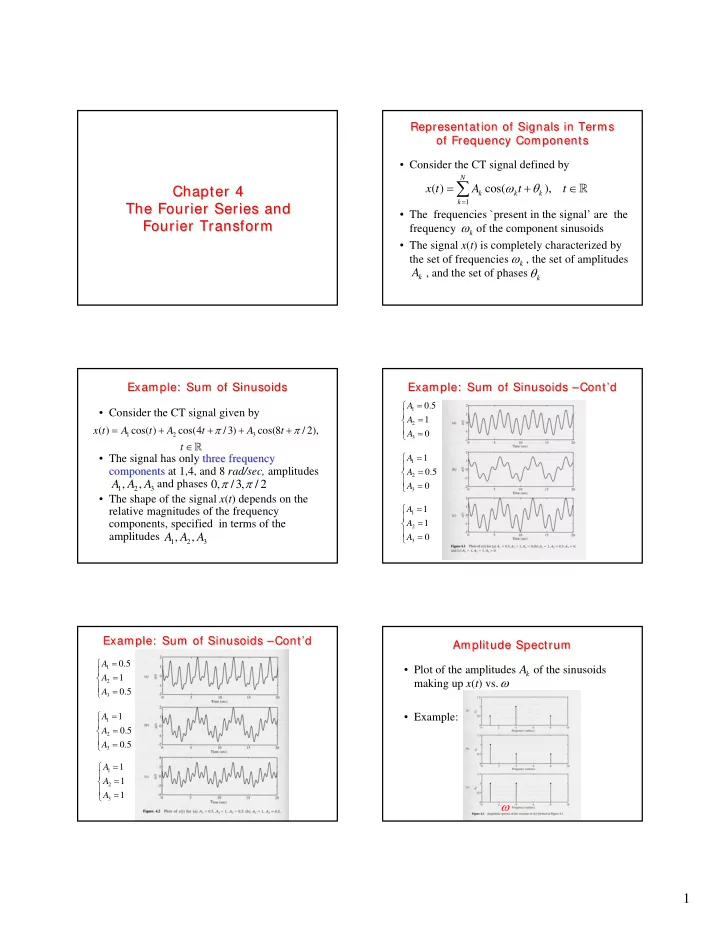
= + ( ) cos( ), x t A t t Chapter 4 Chapter 4 k - PDF document

Representation of Signals in Terms Representation of Signals in Terms of Frequency Components of Frequency Components • Consider the CT signal defined by N ∑ = ω + θ ∈ � ( ) cos( ), x t A t t Chapter 4 Chapter 4 k k k = 1 k The Fourier Series and The Fourier Series and • The frequencies `present in the signal’ are the ω Fourier Transform Fourier Transform frequency of the component sinusoids k • The signal x ( t ) is completely characterized by ω the set of frequencies , the set of amplitudes k θ A , and the set of phases k k Example: Sum of Sinusoids Example: Sum of Sinusoids –Cont’d Example: Sum of Sinusoids Example: Sum of Sinusoids –Cont’d ⎧ = A 0.5 1 • Consider the CT signal given by ⎪ = ⎨ A 1 2 = + + π + + π ⎪ ( ) cos( ) cos(4 /3) cos(8 / 2), x t A t A t A t = ⎩ A 0 1 2 3 3 ∈ � t = ⎧ • The signal has only three frequency three frequency 1 A 1 ⎪ = components components at 1,4, and 8 rad/sec, amplitudes ⎨ 0.5 A 2 π π ⎪ , , and phases 0, /3, / 2 A A A = ⎩ A 0 1 2 3 3 • The shape of the signal x ( t ) depends on the ⎧ = A 1 relative magnitudes of the frequency 1 ⎪ = components, specified in terms of the ⎨ A 1 2 ⎪ = amplitudes , , A A A ⎩ A 0 1 2 3 3 Example: Sum of Sinusoids –Cont’d Example: Sum of Sinusoids –Cont’d Amplitude Spectrum Amplitude Spectrum = ⎧ 0.5 A 1 • Plot of the amplitudes of the sinusoids A ⎪ = k ⎨ A 1 ω 2 making up x ( t ) vs. ⎪ = ⎩ A 0.5 3 ⎧ = • Example: A 1 1 ⎪ = ⎨ A 0.5 2 ⎪ = ⎩ A 0.5 3 ⎧ = A 1 1 ⎪ = ⎨ A 1 2 ⎪ = ⎩ A 1 3 ω 1

Phase Spectrum Phase Spectrum Complex Exponential Form Complex Exponential Form θ • Plot of the phases of the sinusoids α = α + α j • Euler formula Euler formula: cos( ) sin( ) k • e j ω making up x ( t ) vs. • Thus ⎡ ω + θ ⎤ ω + θ = ℜ⎣ j ( t ) cos( ) A t A e k k ⎦ • Example: k k k k real part real part whence N ∑ = ℜ ⎡ ω + θ ⎤ ∈ ( ) j t � ( ) , x t A e t ⎣ k k ⎦ k = 1 k ω Complex Exponential Form – Cont’d Complex Exponential Form – Cont’d Complex Exponential Form – Cont’d Complex Exponential Form – Cont’d ℜ = + z ∗ • And, recalling that where ( ) ( )/ 2 z z = + , we can also write z a jb • By defining N 1 ∑ ⎡ ω + θ − ω + θ ⎤ = + ∈ j ( t ) j ( t ) � ( ) , A A x t A e A e t ⎣ k k k k ⎦ = e θ − = − θ k j j k k k c k c e 2 k = k k k 1 2 2 • This signal contains both positive and it is also negative frequencies N N ∑ ∑ ⎡ ⎤ = ω + − ω = ω ∈ � j t j t j t ( ) , x t c e c e c e t ⎣ k k ⎦ k − ω − k k k • The negative frequencies stem from =− = k 1 k N k writing the cosine in terms of complex ≠ � k � 0 �� � exponentials and have no physical meaning complex exponential form complex exponential form of the signal x ( t ) Line Spectra Line Spectra Example: Line Spectra Example: Line Spectra = + + π + + π ( ) cos( ) 0.5cos(4 /3) cos(8 / 2) • The amplitude spectrum amplitude spectrum of x ( t ) is defined as x t t t t ω the plot of the magnitudes versus | c | k • The phase spectrum phase spectrum of x ( t ) is defined as the 0. ω ∠ = plot of the angles versus c arg( c ) 0. k k • This results in line spectra line spectra which are defined for both positive and negative frequencies k = … • Notice: for 1,2, = ∠ = −∠ | | | | c c − c c − k k k k = − arg( c ) arg( c − ) k k 2

Fourier Series Representation of Fourier Series Representation of The Fourier Series The Fourier Series Periodic Signals Periodic Signals • Then, x ( t ) can be expressed as ∞ • Let x ( t ) be a CT periodic signal with period ∑ = ω ∈ jk t � ( ) , x t c e 0 t + = ∀ ∈ ( ) ( ), T, i.e., x t T x t t R k =−∞ k ω = π 2 / T where is the fundamental fundamental 0 • Example: the rectangular pulse train rectangular pulse train frequency ( rad/sec ) of the signal and frequency / 2 T 1 ∫ − ω = = ± ± jk t … ( ) , 0, 1, 2, c x t e dt k o k T − T / 2 c is called the constant or dc component of x ( t ) 0 The Fourier Series – Cont’d Dirichlet Conditions The Fourier Series – Cont’d Dirichlet Conditions • A periodic signal x ( t ), has a Fourier series k ω • The frequencies present in x ( t ) are 0 if it satisfies the following conditions: integer multiples of the fundamental ω 1. x ( t ) is absolutely absolutely integrable integrable over any frequency 0 period, namely • Notice that, if the dc term c is added to + 0 a T = ∑ N ∫ < ∞ ∀ ∈ c e ω � j t | ( ) | x t dt , a x t ( ) k k =− k N a ≠ k 0 N = ∞ 2. x ( t ) has only a finite number of maxima finite number of maxima and we set , the Fourier series is a and minima over any period and minima special case of the above equation where all ω 3. x ( t ) has only a finite number of finite number of the frequencies are integer multiples of 0 discontinuities over any period discontinuities Example: The Rectangular Pulse Example: The Rectangular Pulse Example: The Rectangular Pulse Train Example: The Rectangular Pulse Train Train – Cont’d Train – Cont’d ∞ 1 1 ∑ − π = + − ∈ |( k 1)/ 2| jk t � ( ) ( 1) , x t e t π 2 k =−∞ k k odd T = ω = π = π 2 2 / 2 • From figure, whence 0 • Clearly x ( t ) satisfies the Dirichlet conditions and thus has a Fourier series representation 3

Trigonometric Fourier Series Trigonometric Fourier Series Example: Trigonometric Fourier Example: Trigonometric Fourier Series of the Rectangular Pulse Train Series of the Rectangular Pulse Train • By using Euler’s formula, we can rewrite ∞ ∑ ω • The expression = ∈ jk t � ( ) , x t c e t 0 ∞ 1 1 k ∑ − π = + − ∈ as =−∞ |( k 1)/ 2| jk t � ( ) ( 1) , k x t e t π ∞ 2 k ∑ =−∞ k = + ω + ∠ ∈ � ( ) 2 | |cos( ), x t c c k t c t �� � ��� � 0 0 k odd k k = can be rewritten as k 1 dc component dc component k k - -th th harmonic harmonic π ∞ ⎛ ⎞ 1 2 ∑ ⎡ − ⎤ = + π + − − ∈ ( k 1)/ 2 � ( ) cos ⎜ ( 1) 1 ⎟ , x t k t t ⎣ ⎦ π ⎝ ⎠ • This expression is called the trigonometric trigonometric 2 k 2 = k 1 Fourier series of x ( t ) Fourier series k odd Gibbs Phenomenon Gibbs Phenomenon Gibbs Phenomenon – Cont’d Gibbs Phenomenon – Cont’d • Given an odd positive integer N, define the 3 ( ) x t 9 ( ) x t N -th partial sum of the previous series π ⎛ ⎞ N 1 2 ∑ ⎡ ⎤ = + π + − − − ∈ ( k 1)/ 2 � ( ) cos ( 1) 1 , x t ⎜ k t ⎟ t ⎣ ⎦ π N ⎝ ⎠ 2 k 2 = 1 k k odd • According to Fourier Fourier’ ’s theorem s theorem, it should be − = lim | ( ) ( ) | 0 x t x t N →∞ N Parseval’s Theorem Parseval’s Theorem Gibbs Phenomenon – Cont’d Gibbs Phenomenon – Cont’d • Let x ( t ) be a periodic signal with period T x 21 ( ) t 45 ( ) x t • The average power average power P of the signal is defined as T / 2 1 ∫ = 2 ( ) P x t dt T − T / 2 ∞ ∑ ω = ∈ jk t � • Expressing the signal as ( ) , x t c e 0 t k =−∞ k it is also ∞ = ∑ 2 | | P c k overshoot: about 9 % of the signal magnitude overshoot =−∞ k N → ∞ (present even if ) 4