cos c a cos a sin f a cos a sin 1
play

+ = + cos( c ) a cos a sin = + f ( ) a - PDF document

Announcements Fourier Transform Send email to the TA for the mailing list Analytic geometry gives a coordinate aster@ umiacs . umd . edu system for describing geometric objects. For problem set 1: turn in written answers to Fourier


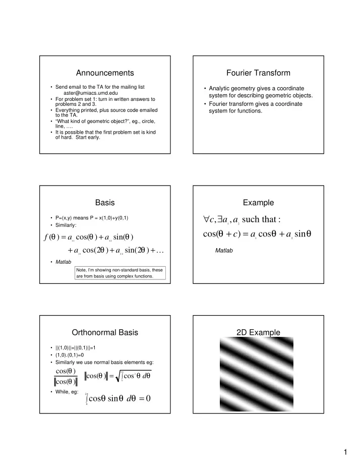
  1. Announcements Fourier Transform • Send email to the TA for the mailing list • Analytic geometry gives a coordinate aster@ umiacs . umd . edu system for describing geometric objects. • For problem set 1: turn in written answers to • Fourier transform gives a coordinate problems 2 and 3. • Everything printed, plus source code emailed system for functions. to the TA. • “What kind of geometric object?”, eg ., circle, line, …. • It is possible that the first problem set is kind of hard. Start early. Basis Example ∀ ∃ • P=(x,y) means P = x(1,0)+y(0,1) c , a , a such that : • Similarly: 1 2 θ + = θ + θ cos( c ) a cos a sin θ = θ + θ f ( ) a cos( ) a sin( ) 1 2 1 1 1 2 + θ + θ + a cos( 2 ) a sin( 2 ) Matlab 2 1 2 2 • Matlab Note, I’m showing non - standard basis, these are from basis using complex functions. Orthonormal Basis 2D Example • ||(1,0)||=||(0,1)||=1 • (1,0).(0,1)=0 • Similarly we use normal basis elements eg : θ cos( ) θ = π θ θ 2 cos( ) ∫ cos 2 d θ cos( ) 0 • While, eg : θ θ θ = π 2 ∫ cos sin d 0 0 1

  2. Remember Convolution Convolution Theorem X X X X X X 11 10 0 0 1 10 ⊗ = 10 X X − 9 10 1 0 1 f g T F * G 11 1 O X X 10 9 10 0 2 1 I X X 11 10 9 9 11 10 F X X 9 10 11 9 99 11 • F,G are transform of f,g X X X X X X 10 9 9 11 10 10 1 1 1 That is, F contains coefficients, when 1 1 1 1/9 we write f as linear combinations of 1 1 1 harmonic basis. 1/9.(10x1 + 11x1 + 10x1 + 9x1 + 10x1 + 11x1 + 10x1 + 9x1 + 10x1) = 1/9.( 90) = 10 Examples Examples θ ⊗ θ = cos cos ? • Transform of box filter is θ ⊗ θ = cos cos 2 ? sinc . • Transform of θ ⊗ = cos f ? Gaussian is Gaussian. θ + θ + θ ⊗ = (cos . 2 cos 2 . 1 cos 3 ) f ? ( Trucco and Verri ) 2

  3. Example: Smoothing by Implications Averaging • Smoothing means removing high frequencies. This is one definition of scale. • Sinc function explains artifacts. • Need smoothing before subsampling to avoid aliasing. Smoothing with a Gaussian Sampling Boundary Detection - Edges • Boundaries of objects – Usually different materials/orientations, intensity changes. 3

  4. We also get: Boundaries of materials Boundaries of surfaces properties Boundaries of lighting Edge is Where Change Occurs • Change is measured by derivative in 1D • Biggest change, derivative has maximum magnitude • Or 2 nd derivative is zero. Noisy Step Edge Optimal Edge Detection: Canny • Gradient is high everywhere. • Assume: • Must smooth before taking gradient. – Linear filtering – Additive iid Gaussian noise • Edge detector should have: – Good Detection. Filter responds to edge, not noise. – Good Localization: detected edge near true edge. – Single Response: one per edge. 4

  5. So, 1D Edge Detection has Optimal Edge Detection: Canny (continued) steps: 1. Filter out noise: convolve with • Optimal Detector is approximately Gaussian Derivative of Gaussian. 2. Take a derivative: convolve with • Detection/Localization trade - off [- 1 0 1] – More smoothing improves detection 3. Find the peak. – And hurts localization. • Matlab • This is what you might guess from • We can combine 1 and 2. (detect change) + (remove noise) • Matlab 5

  6. This document was created with Win2PDF available at http://www.daneprairie.com. The unregistered version of Win2PDF is for evaluation or non-commercial use only.

Download Presentation
Download Policy: The content available on the website is offered to you 'AS IS' for your personal information and use only. It cannot be commercialized, licensed, or distributed on other websites without prior consent from the author. To download a presentation, simply click this link. If you encounter any difficulties during the download process, it's possible that the publisher has removed the file from their server.

Recommend


More recommend