Contributions 1. Understandable visualizations using optimization on - - PowerPoint PPT Presentation

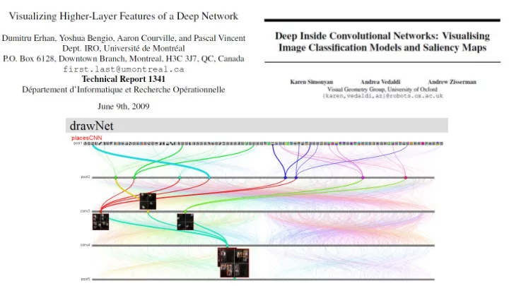
Contributions

• 1. Understandable visualizations using optimization on the input image [ Similar to Activation

Maximization, only applied to ImageNet]

• 2. Compute a spatial support of a given class in a given image
• 3. Relation DeConv Networks [Zeiler and Fergus, 2013]

Class Model Visualization

Objective

Generating an image which is representative of the class in terms of a Class Scoring Model Sc(I): Score of class c for an image I, we want to solve the following optimization problem

 

2 2

arg max I

c

S I I  

Method

Initialize with a zero image then backprop through the network to find the image instead of adjusting weights.

Class Model Visualization

Numerically computed images, illustrating the class appearance models, learnt by a ConvNet, trained on ILSVRC-2013. Note how different aspects of class appearance are captured in a single image.

Slide Credits: Simonyan et al. 2014

Class Model Visualization

Maximize the score and not the posterior probability Maximizing Score: Simonyan et al. 2014 Maximizing Probability: Nguyen et al. 2015

Image Specific Class Saliency Visualization

Objective

Rank the pixels in image I0 in the order of their influence in the class score Sc for class c

 

T c c c

S I w I b  

Linear Model (Motivating Example)

Score Models

In this case, with Deep Conv Nets, Sc is a highly non-linear function of I

Solution

Image Specific Class Saliency Visualization

 

T c

S I w I b  

where,

c I

S w I   

Taylor Series Expansion, Local Linearity

Score Models

w is found by back prop and the saliency map is computed by:

( , ) ij h i j

M w 

( , , )

max

ij c h i j c

M w 

GrayScale MultiChannel

      

'

f x f x f x x x   

For our case

where h(i,j) is the index of the vector w corresponding to the image pixel in the i-th row and j-th column

Image Specific Class Saliency Visualization

Slide Credit: Simonyan et al. 2014

Weakly Supervized Object Localization

Slide Credits: Simonyan ILSVRC 2013

• Given an image and a saliency map

Weakly Supervized Object Localization

Slide Credits: Simonyan ILSVRC 2013

• Given an image and a saliency map
• 1. Foreground/Background mask using thresholds
• n saliency. (Foreground > 95% quantile and

Background < 30% quantile of saliency distribution)

Weakly Supervized Object Localization

Slide Credits: Simonyan ILSVRC 2013

• Given an image and a saliency map
• 1. Foreground/Background mask using thresholds
• n saliency. (Foreground > 95% quantile and

Background < 30% quantile of saliency distribution)

• 2. GraphCut Color Segmentation

[Boykov and Jolly, 2001]

Weakly Supervized Object Localization

Slide Credits: Simonyan ILSVRC 2013

• Given an image and a saliency map
• 1. Foreground/Background mask using thresholds
• n saliency. (Foreground > 95% quantile and

Background < 30% quantile of saliency distribution)

• 2. GraphCut Color Segmentation

[Boykov and Jolly, 2001]

• 3. Bounding Box of largest connected component.

ILSVRC – 2013: Achieved a Top-5 Localization Error of 46.4 % with this weakly supervised

• approach. (Challenge winner had 29.9% with a

supervised approach)

Relation to DeConvulation Networks and

Slide Credits: Simonyan et al ICLR Workshop 2014

Goal

• 1. To visualize what a unit computes in an arbitrary layer of a deep network in the input image

space

• 2. Generalizing the method so that it is applicable to different models

Activation Maximization

Objective Look for input patterns which maximize the activation of the i-th neuron of j-th layer

 

*

arg max ,

ij x

x h x









Sampling from a Deep Belief Network

• 1. Clamp the unit hij to 1.
• 2. Sample inputs x by performing ancestral top-down sampling going from layer j-1 to input.
• 3. Produces a conditional distribution
• 4. Characterize the unit hij by computing

 

| 1

j ij

p x h  | 1

ij

E x h     

Experiment Setup

Datasets

• 1. Extended MNIST Dataset, Loosli et al., 2007: 2.5 Million 28x28 Grayscale Images
• 2. Nautral Image Patches, Olshaushen and Field, 1996: 100000 12x12 Patches of whitened natural image patches

For Activation Maximization

Random Test vector sampled from [0,1] of dimensions 28x28 or 12x12 and gradient ascent is applied. Re-normalization of x* to the average norm of the dataset is done.

Networks

• 1. Deep Belief Networks (DBN), Hinton et al. (2006)
• 2. Stacked Denoising Auto-Encoders, Vincent et al. (2007)

Activation Maximization

Slide Credit: Erhan et al. (2009)

Sensitivity Analysis The post-sigmoidal activation

• f unit j (columns) when the

input to the network is the “optimal” pattern i (rows)

Activation Maximization

Slide Credit: Erhan et al. (2009)

Comparison of Different Methods

Slide Credit: Erhan et al. (2009)

Demo

• 1. Drawnet: http://people.csail.mit.edu/torralba/research/drawCNN/drawNet.html
• 2. DeepVis: https://www.youtube.com/watch?v=AgkfIQ4IGaM