Constraints on radial anisotropy in the central Pacific upper mantle - PowerPoint PPT Presentation

� S14A-05 � Constraints on radial anisotropy in the central Pacific upper mantle from the NoMelt OBS array Joshua B. Russell 1 , James B. Gaherty 1 , Peiying (Patty) Lin 2 , Molly Zebker 1 1 Lamont-Doherty Earth Observatory, Columbia University 2 Taiwan Ocean Research Institute, Kaohsiung, Taiwan

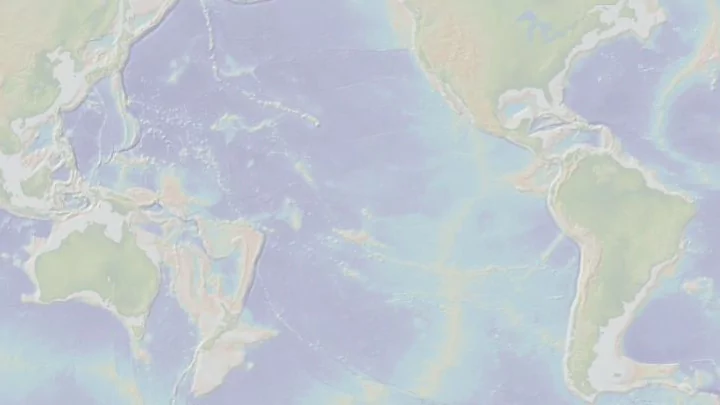
NoMelt Experiment 160 ˚ W 150 ˚ W 140 ˚ W 25 ˚ N 25 ˚ N Situated on relatively pristine oceanic lithosphere (~70 Ma) 60 Ma 20 ˚ N 20 ˚ N One year of continuous data collected in 70 Ma 8 0 2012 M a 15 ˚ N 15 ˚ N 600x400 km footprint – 16 broad-band OBS 10 ˚ N 10 ˚ N – Short-period OBS 5 ˚ N 5 ˚ N – Magnetotelluric array 0 ˚ 0 ˚ 160 ˚ W 150 ˚ W 140 ˚ W

Motivation • Azimuthal and radial anisotropy constrain flow patterns within the mantle • Previous observations of anisotropy in the lithosphere beneath ocean basins are Radial consistent with horizontally Anisotropy aligned olivine fabric associated Azimuthal with seafloor spreading V SH > V SV Anisotropy • Inconsistencies remain between recent regional and global models of radial anisotropy in the lithosphere NoMelt provides new constraints on Pacific mantle anisotropy, measured at a local scale. Nishimura & Forsyth, 1989 �

NoMelt azimuthal anisotropy Azimuthal variation of Rayleigh wave phase velocities oriented parallel to the fossil spreading direction (~78º) in the lithosphere V SV G Amplitude Fast Direction • Strong anisotropy in lid oriented parallel to FSD • Weak anisotropy in the low velocity zone (100-150 km) • Stronger anisotropy below the LVZ associated with asthenospheric flow How does strength of radial anisotropy beneath the central Pacific compare with azimuthal Lin et al., Nature (2016) � anisotropy? PeiYing (Patty) Lin: [S21C-05] Tues. 9-9:15 Room 307

Motivation: Radial anisotropy Central Pacific Models 0 0 • Radial anisotropy ξ is also important for constraining upper-mantle circulation and evolution of the 50 50 lithosphere-asthenosphere system 100 100 • Radial anisotropy may reflect Depth (km) processes controlling the G 150 150 discontinuity • Discrepancies exist between current 200 200 models of radial anisotropy in the central Pacific upper-mantle Beghein 2014 250 250 NF 52 − 110 Ma • Requires constraints from both Love S362WMANI+M Pa5 and Rayleigh waves NoMelt SV 300 300 3.5 4 4.5 5 0.9 1 1.1 V SV (km/s) ξ = (V SH /V SV ) 2

Method Ambient noise provides constraints from both Rayleigh and Love wave fields Phase velocities derived from waveform fitting of ambient-noise cross spectra [ Menke & Jin, BSSA 2015 ] SNR : 2.3127 Distance : 540.6619km Data 0.02 Synthetic 0.01 cross spectra: 0 − 0.01 240 cross-correlation functions − 0.02 0.1 0.15 0.2 0.25 Frequency (Hz) B01 − B24 Phase Velocity (km/s) 4.6 4.4 Starting Model 4.2 Fit 4 3.8 4 5 6 7 8 9 10 Period (s)

1 st overtone Rayleigh waves (4-10 s) Cross spectral power All stations Z • Sensitivity of 1 st overtone Rayleigh comparable − 80 mean to fundamental mode Love wave − 100 Power • Strong 2 θ azimuthal signal − 120 – Rayleigh fast direction parallel to fossil − 140 1 2 10 10 spreading (78º) Period (s) All stations Z Vertical 4-10 s 0 water 2 θ Anisotropy column 100 10 s 8.6 s 7.5 s 6.7 s 10 s 8.5714 s 7.5 s 6.6667 s 4 4 4 4 200 c/c (%) Distance (km) 2 2 2 2 4 0 0 0 0 δ c/c (%) − 2 − 2 − 2 − 2 2 300 − 4 − 4 − 4 − 4 − 100 0 100 − 100 0 100 − 100 0 100 − 100 0 100 0 6 s 5.5 s 5 s 4.6 s 6 s 5.4545 s 5 s 4.6154 s 400 − 2 4 4 4 4 2 2 2 2 500 0 0 0 0 − 2 − 2 − 2 − 2 1 st overtone − 4 − 4 − 4 − 4 − 100 0 100 − 100 0 100 − 100 0 100 − 100 0 100 600 − 100 0 100 Azimuth (degrees) − 200 − 100 0 100 200 Azimuth (degrees) lag time (s) 4 s

Fundamental mode Love waves (4-10 s) Cross spectral power All stations T − 80 • Clear 4 θ azimuthal signal mean Power − 100 – Love slow direction parallel to fossil − 120 spreading (78º) − 140 1 2 – 10 10 Consistent with predictions of olivine fabric Period (s) All stations T T : All non − repeated pairs, filtered at 4 − 10(s) Transverse 4-10 s 0 4 θ Anisotropy 100 10 s 8.6 s 7.5 s 6.7 s 10 s 8.5714 s 7.5 s 6.6667 s 4 4 4 4 200 c/c (%) Distance (km) 2 2 2 2 4 0 0 0 0 δ c/c (%) − 2 − 2 − 2 − 2 2 300 − 4 − 4 − 4 − 4 − 100 0 100 − 100 0 100 − 100 0 100 − 100 0 100 0 6 s 5.5 s 5 s 4.6 s 6 s 5.4545 s 5 s 4.6154 s 400 − 2 4 4 4 4 2 2 2 2 500 0 0 0 0 − 2 − 2 − 2 − 2 − 4 − 4 − 4 − 4 − 100 0 100 − 100 0 100 − 100 0 100 − 100 0 100 600 − 100 0 100 Azimuth (degrees) − 200 − 100 0 100 200 Azimuth (degrees) lag time (s) 4 s

Measurements Phase Velocity (km/s) 4.5 Strong azimuthal anisotropy 4 Isotropic suggests significant mantle 3.5 phase veloc. sensitivity Fund. mode Love Rayleigh S1 Rayleigh S0 Fund. mode Rayleigh 3 1 st overtone Rayleigh Love T0 NoMelt SV NoMelt 2.5 1 10 Fréchet Kernels (5-7.5 s) Peak − to − peak amp (%) 5 4 θ Love SV SH 4 2 θ Rayleigh Azimuthal 0 0 3 anisotropy 2 (%) 5 5 1 0 1 Depth (km) Depth (km) 10 10 10 4 θ slow 15 15 150 Fast Direction 2 θ fast FSD ~78º Azimuth 100 20 20 (º) Fund. mode Love 50 Rayleigh S1 1 st overtone Rayleigh Love T0 25 25 0 0 1 2 0 1 2 1 10 − 7 − 7 x 10 x 10 Period (s)

Inversion Solving for horizontal and vertical Crustal Model PV SV V P & V S 4 4 V P V S 5 5 Starting model 6 6 V P 7 7 Depth (km) Depth (km) 0-35km: NoMelt refraction model accounting for ~8% P-azimuthal 8 8 anisotropy in the mantle (D. Lizarralde personal communications) 9 9 V S 10 10 Sediments: Seafloor compliance 11 11 [ Ruan et al., JGR 2014 ] NoMelt SV NoMelt Crust: V P /V S = ~1.85 [ Brocher, BSSA 2005 ] 12 12 crust1.0 Starting model Mantle: NoMelt SV [ Lin et al., Nature 2016 ] 13 13 0 2 4 6 0 2 4 V P (km/s) V S (km/s)

Inversion results V SH > V SV required in the mantle lithosphere and cannot be ruled out in the crust Fit to data V SV V SV Anisotropy Anisotropy Rayleigh Love 4 4 4.2 Phase velocity (km/s) 4.4 6 6 4 4.3 8 8 ~ 2% 4.2 3.8 4.1 10 10 Observed Depth (km) 3.6 4 5 6 7 5 6 7 12 12 ~ 5% Rayleigh Residual Love Residual 14 14 2 σ error 1 1 16 16 δ c % 0 0 18 18 Starting Model − 1 − 1 starting 20 20 3 4 5 1 1.1 1.2 5 6 7 5 6 7 V (km/s) ξ = (V SH /V SV ) 2 Periods (s) Periods (s)

Summary & Interpretation Both azimuthal and radial anisotropy required in the lithospheric mantle To Ridge Mantle FSD Ø Radial anisotropy: V SH > V SV (~ 3-7%) 4 θ slow Ø Clear 2 θ and 4 θ azimuthal anisotropy • Consistent with petrologic models of olivine 2 θ fast with orthorhombic or hexagonal symmetry • Horizontal preferred alignment of olivine a- axis associated with fossil spreading V SH > V SV ? ¡ 0 - 5 % Crust V SH > V SV Ø V SH > V SV (0-5%) 3 - 7% a-axis • Horizontal crustal fabric? ? ¡ – Layering processes? Cracks? Fluids?

Additional inversions: Good fits V SV Anisotropy Rayleigh Love 4 4 4.2 Phase velocity (km/s) 4.4 6 6 4 4.3 8 8 4.2 3.8 4.1 10 10 Depth (km) 3.6 4 5 6 7 8 5 6 7 8 12 12 Rayleigh Residual Love Residual 14 14 1 1 16 16 δ c % 0 0 18 18 − 1 − 1 20 20 1 1.1 1.2 3 4 5 5 6 7 8 5 6 7 8 ξ = (V SH /V SV ) 2 V (km/s) Periods (s) Periods (s)

Additional inversions: Poor fits V SV Anisotropy Rayleigh Love 4 4 4.2 Phase velocity (km/s) 4.4 6 6 4 4.3 8 8 4.2 3.8 4.1 10 10 Depth (km) 3.6 4 5 6 7 8 5 6 7 8 12 12 Rayleigh Residual Love Residual 14 14 1 1 16 16 δ c % 0 0 starting 18 18 iso mantle iso crust + mantle − 1 − 1 fixed crust 20 20 1 1.1 1.2 3 4 5 5 6 7 8 5 6 7 8 ξ = (V SH /V SV ) 2 V (km/s) Periods (s) Periods (s)

Kernel Nonlinearity: Love waves (20-100 s) Love Waves (20-100 s) 201202021334 20.5km 57 56 Distance (degrees) 55 54 53 52 51 900 1000 1100 1200 1300 1400 1500 1600 Seconds

Kernel Nonlinearity: 4-30 s Rayleigh Love 1 st overtone Fundamental Mode Velocity Model 0 0 0 50 50 50 100 100 100 5 s 5 S Depth (km) 5.4545 s 5.4545 S 6 s 6 S 150 150 6.6667 s 150 6.6667 S 7.5 s 7.5 S 8.5714 s 8.5714 S 10 s 10 S 12 s 12 S 200 200 200 12.8571 s 12.8571 S 13.8462 s 13.8462 S 15 s 15 S 16.3636 s 16.3636 S 18 s 18 S 250 250 250 20 s 20 S 22.5 s 22.5 S 25.7143 s 25.7143 S 30 s 30 S 300 300 300 3 4 5 0 2 4 0 2 4 V SH (km/s) − 8 − 8 x 10 x 10