Concavity MCV4U: Calculus & Vectors Consider the graph of y = x - PDF document

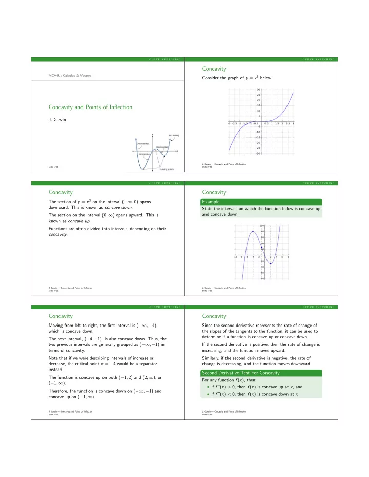
c u r v e s k e t c h i n g c u r v e s k e t c h i n g Concavity MCV4U: Calculus & Vectors Consider the graph of y = x 3 below. Concavity and Points of Inflection J. Garvin J. Garvin — Concavity and Points of Inflection Slide 1/21 Slide 2/21 c u r v e s k e t c h i n g c u r v e s k e t c h i n g Concavity Concavity The section of y = x 3 on the interval ( −∞ , 0) opens Example downward. This is known as concave down . State the intervals on which the function below is concave up and concave down. The section on the interval (0 , ∞ ) opens upward. This is known as concave up . Functions are often divided into intervals, depending on their concavity . J. Garvin — Concavity and Points of Inflection J. Garvin — Concavity and Points of Inflection Slide 3/21 Slide 4/21 c u r v e s k e t c h i n g c u r v e s k e t c h i n g Concavity Concavity Moving from left to right, the first interval is ( −∞ , − 4), Since the second derivative represents the rate of change of which is concave down. the slopes of the tangents to the function, it can be used to determine if a function is concave up or concave down. The next interval, ( − 4 , − 1), is also concave down. Thus, the two previous intervals are generally grouped as ( −∞ , − 1) in If the second derivative is positive, then the rate of change is terms of concavity. increasing, and the function moves upward. Note that if we were describing intervals of increase or Similarly, if the second derivative is negative, the rate of decrease, the critical point x = − 4 would be a separator change is decreasing, and the function moves downward. instead. Second Derivative Test For Concavity The function is concave up on both ( − 1 , 2) and (2 , ∞ ), or For any function f ( x ), then: ( − 1 , ∞ ). • if f ′′ ( x ) > 0, then f ( x ) is concave up at x , and Therefore, the function is concave down on ( −∞ , − 1) and • if f ′′ ( x ) < 0, then f ( x ) is concave down at x concave up on ( − 1 , ∞ ). J. Garvin — Concavity and Points of Inflection J. Garvin — Concavity and Points of Inflection Slide 5/21 Slide 6/21

c u r v e s k e t c h i n g c u r v e s k e t c h i n g Concavity Concavity Example Use the quotient rule again to determine the second derivative. Show that the function f ( x ) = x + 2 is concave down on f ′′ ( x ) = x 3 − 3 x 2 ( x + 4) x 2 ( −∞ , − 6) and concave up on ( − 6 , 0) ∪ (0 , ∞ ). x 6 = − 2( x + 6) Find the first derivative using the quotient rule. x 4 f ′ ( x ) = x 2 − 2 x ( x + 2) Test values in the intervals ( −∞ , − 6), ( − 6 , 0) and (0 , ∞ ). x 4 Interval ( −∞ , − 6) ( − 6 , 0) (0 , ∞ ) = − x + 4 x − 7 − 1 1 x 3 2 f ′′ ( x ) 10 14 − 2401 sign + + − Therefore, f ( x ) is concave down on ( −∞ , − 6) and concave up elsewhere. J. Garvin — Concavity and Points of Inflection J. Garvin — Concavity and Points of Inflection Slide 7/21 Slide 8/21 c u r v e s k e t c h i n g c u r v e s k e t c h i n g Concavity Points of Inflection A graph of f ( x ) suggests that these intervals are valid. What happens if f ′′ ( x ) = 0? Evaluating the previous example at x = − 6 gives f ′′ ( − 6) = 2( − 6+6) = 0, which is neither concave up nor ( − 6) 4 concave down. A point at which a function changes concavity (from concave up to concave down, or vice versa ) is called a point of inflection . Like critical values, points of inflection may occur for values of x where f ′′ ( x ) = 0, or f ′′ ( x ) is undefined. Since f ( − 6) = − 1 � − 6 , − 1 � 9 , there is a point of inflection at 9 in the previous example. J. Garvin — Concavity and Points of Inflection J. Garvin — Concavity and Points of Inflection Slide 9/21 Slide 10/21 c u r v e s k e t c h i n g c u r v e s k e t c h i n g Points of Inflection Points of Inflection A graph of y = x 3 + 3 x 2 − 9 x − 8 shows how the function Example changes from concave down to concave up at ( − 1 , 3). Determine any points of inflection for the function y = x 3 + 3 x 2 − 9 x − 8. dx = 3 x 2 + 6 x − 9, and the second The derivative is dy derivative is d 2 y dx 2 = 6 x + 6 = 6( x + 1). Since 6( x + 1) = 0 when x = − 1, a point of inflection should occur at this value. When x = − 1, y = ( − 1) 3 + 3( − 1) 2 − 9( − 1) − 8 = 3, so ( − 1 , 3) is a point of inflection. J. Garvin — Concavity and Points of Inflection J. Garvin — Concavity and Points of Inflection Slide 11/21 Slide 12/21

c u r v e s k e t c h i n g c u r v e s k e t c h i n g Points of Inflection Points of Inflection The conditions “ f ′′ ( x ) = 0” and “ f ′′ ( x ) is undefined” are not Example sufficient to ensure a point of inflection at x . Determine any points of inflection for the function f ( x ) = x 4 . Recall that the second derivative represents the rate of The derivative is f ′ ( x ) = 4 x 3 , and the second derivative is change of the slopes of the tangents. f ′′ ( x ) = 12 x 2 . If the slopes change from positive to negative at x , then x Since 12 x 2 = 0 when x = 0, this suggests a point of might represent a local maximum. Such an interval would be inflection at (0 , 0). Testing on either side of x = 0, however, entirely concave down. shows that f ( x ) is concave up everywhere on its domain. Similarly, if the slopes change from negative to positive at x , a local minimum may occur at x and the corresponding Interval ( −∞ , 0) (0 , ∞ ) interval would be concave up. − 1 1 x f ′′ ( x ) 12 12 sign + + Therefore, (0 , 0) is a local minimum. J. Garvin — Concavity and Points of Inflection J. Garvin — Concavity and Points of Inflection Slide 13/21 Slide 14/21 c u r v e s k e t c h i n g c u r v e s k e t c h i n g Points of Inflection Classifying Extrema Since f ( x ) = x 4 is an even-degree power function with a In the previous example, the second derivative was zero at positive leading coefficient, it is concave up on ( −∞ , ∞ ). x = 0, but there was no inflection point. Most of the time, the second derivative can tell us if there is a local minimum or local maximum at a given point. Second Derivative Test For Extrema If x is a critical point for f ( x ), then: • there is a local maximum at x if f ′′ ( x ) < 0, and • there is a local minimum at x if f ′′ ( x ) > 0. If f ′′ ( x ) = 0, as in the previous example, then there may be a local extremum at x , or there may not be. J. Garvin — Concavity and Points of Inflection J. Garvin — Concavity and Points of Inflection Slide 15/21 Slide 16/21 c u r v e s k e t c h i n g c u r v e s k e t c h i n g Classifying Extrema Classifying Extrema When x = 0, dy Example dx is undefined, so there is a vertical asymptote at x = 0. Use the second derivative to determine the nature of the critical points of y = x 2 + 4 Find the second derivative using the quotient rule again. . 2 x dx 2 = 2 x (2 x 2 ) − 4 x ( x 2 − 4) d 2 y Determine the first derivative using the quotient rule. 4 x 4 = 4 dx = 2 x (2 x ) − 2( x 2 + 4) dy x 3 4 x 2 = x 2 − 4 Since f ′′ ( − 2) = − 1 2 < 0, the graph is concave down on the 2 x 2 interval containing x = − 2, so there is a local maximum = ( x − 2)( x + 2) when x = − 2. 2 x 2 Similarly, since f ′′ (2) = 1 2 > 0, the graph is concave up on the interval containing x = 2, so there is a local minimum Therefore, critical points occur at x = 0 and x = ± 2. when x = − 2. J. Garvin — Concavity and Points of Inflection J. Garvin — Concavity and Points of Inflection Slide 17/21 Slide 18/21

c u r v e s k e t c h i n g c u r v e s k e t c h i n g Classifying Extrema Classifying Extrema A graph is below. Note that since d 2 y dx 2 can never equal 0, The same conclusion could be reached using the first there are no points of inflection. derivative instead. Divide the function into four intervals (between critical points and asymptotes) and test values. Interval ( −∞ , − 2) ( − 2 , 0) (0 , 2) (2 , ∞ ) x − 3 − 1 1 3 5 − 3 − 3 5 f ′ ( x ) 18 2 2 18 sign + − − + Since f ′ ( x ) changes from positive to negative at x = − 2, the function changes from increasing to decreasing at that point. Therefore, there is a local maximum at x = − 2. Similarly, the change from negative to positive at x = 2 indicates a local minimum at x = 2. J. Garvin — Concavity and Points of Inflection J. Garvin — Concavity and Points of Inflection Slide 19/21 Slide 20/21 c u r v e s k e t c h i n g Questions? J. Garvin — Concavity and Points of Inflection Slide 21/21