Concatenation and Kleene Star on Deterministic Finite Automata - - PDF document

SLIDE 1

Concatenation and Kleene Star

• n Deterministic Finite Automata

Guo-Qiang Zhang∗, Xiangnan Zhou†, Robert Fraser‡, Licong Cui∗

∗Department of Electrical Engineering and Computer Science, Case Western Reserve University, Cleveland, Ohio 44106, USA

Email: {gq, licong.cui}@case.edu

†College of Mathematics and Econometrics, Hunan University, Changsha 410012, China Email: xnzhou81026@163.com ‡Department of Mathematics, Case Western Reserve University, Cleveland, Ohio 44106, USA Email: rgf11@case.edu

Abstract—This paper presents direct, explicit algebraic con- structions of concatenation and Kleene star on deterministic finite automata (DFA), using the Boolean-matrix method of Zhang [5] and ideas of Kozen [2]. The consequence is trifold: (1) it provides an alternative proof of the classical Kleene’s Theorem

• n the equivalence of regular expressions and DFAs without using

nondeterministic finite automata (NFA); (2) it demonstrates how the language constructions of concatenation and Kleene star can be captured elegantly as algebraic laws in the form of “binomial theorems;” (3) it provides a demonstration of the (tight) upper bounds of the state complexity of concatenation and Kleene star, but offers a way to study the state complexity of NFA also.

• I. MATRIX-APPROACH TO AUTOMATA THEORY

A Boolean matrix is a matrix (of size m×n) whose elements are either 0 or 1, where the internal operations are carried out

• ver the Boolean algebra. We write Bm×n for the set of all

Boolean matrices of size m × n. A Boolean (row) vector of dimension n is an n-tuple (b1, b2, . . . , bn) of 0s and 1s. We write Bn for the set of all Boolean vectors of dimension n. A column vector is the transpose ( )t of a row vector. The characteristic vector of a subset A of {1, · · · , n} is the row vector In

A ∈ Bn such that the p-th component of In A is a 1

if and only if p ∈ A. The characteristic vector of a singleton set {p} is written as In

p, or simply Ip. Om×n stands for an

(m × n)-matrix, all of its elements are 0. When dimension is fixed by context, we abuse notion and write On×n as 0. A deterministic finite automaton (DFA) is a 5-tuple M = (Q, Σ, δ, q0, F), where Q is the finite set of states, Σ is the alphabet, δ : Q × Σ → Q is the transition function, q0 is the start state, and F is the set of final states. For notational convenience, we use initial segments of natural numbers {1, 2, · · · , n} to denote the set of states, and fix 1 to be the start state, for base/background DFAs. When there is no confusion, we omit the indication of the start state (which is assumed to be state 1 by default). Each n-state DFA determines a (associated) matrix system {∆a | a ∈ Σ}, where ∆a is the (n × n) adjacency matrix

• f the a-labeled subgraph associated with the DFA. In other

words, the (i, j) entry of ∆a is 1 if and only if δ(i, a) = j. Since M is a DFA, each ∆a is row-stochastic (i.e., every row contains precisely a single 1). The (Boolean) sum ∆ of all members ∆a in the matrix system is the adjacency matrix. For a string w = a1a2 · · · an over Σ, we write ∆w for the matrix product ∆a1∆a2 · · · ∆an. The language accepted by M, denoted L(M), is the set {w | Iq0∆wIt

F = 1}. We refer

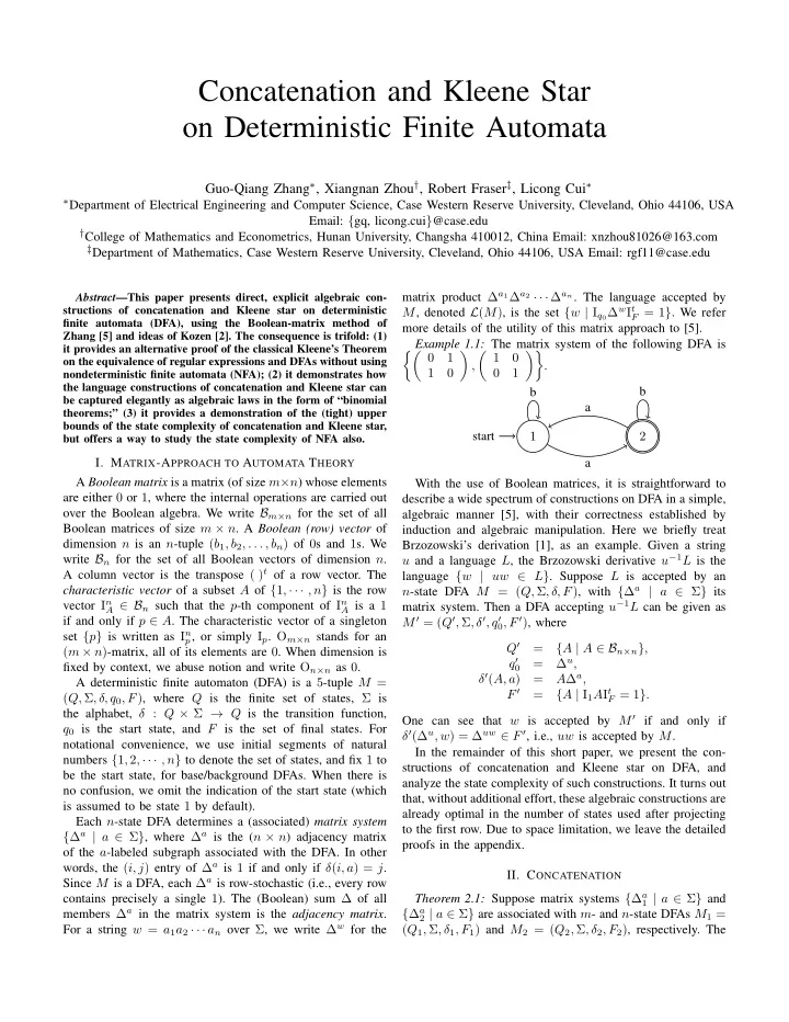
more details of the utility of this matrix approach to [5]. Example 1.1: The matrix system of the following DFA is 1 1

• ,

1 1

• .

1 start 2 b a a b With the use of Boolean matrices, it is straightforward to describe a wide spectrum of constructions on DFA in a simple, algebraic manner [5], with their correctness established by induction and algebraic manipulation. Here we briefly treat Brzozowski’s derivation [1], as an example. Given a string u and a language L, the Brzozowski derivative u−1L is the language {w | uw ∈ L}. Suppose L is accepted by an n-state DFA M = (Q, Σ, δ, F), with {∆a | a ∈ Σ} its matrix system. Then a DFA accepting u−1L can be given as M ′ = (Q′, Σ, δ′, q′

0, F ′), where

Q′ = {A | A ∈ Bn×n}, q′ = ∆u, δ′(A, a) = A∆a, F ′ = {A | I1AIt

F = 1}.

One can see that w is accepted by M ′ if and only if δ′(∆u, w) = ∆uw ∈ F ′, i.e., uw is accepted by M. In the remainder of this short paper, we present the con- structions of concatenation and Kleene star on DFA, and analyze the state complexity of such constructions. It turns out that, without additional effort, these algebraic constructions are already optimal in the number of states used after projecting to the first row. Due to space limitation, we leave the detailed proofs in the appendix.

• II. CONCATENATION

Theorem 2.1: Suppose matrix systems {∆a

1 | a ∈ Σ} and

{∆a

2 | a ∈ Σ} are associated with m- and n-state DFAs M1 =

(Q1, Σ, δ1, F1) and M2 = (Q2, Σ, δ2, F2), respectively. The

SLIDE 2

DFA M = (Q, Σ, δ, q0, F) defined as Q = {(A, B) | A ∈ Bm×m, B ∈ Bm×n}, q0 = (T 0, T), δ((A, B), a) = (A, B)∆a (= (A∆a

1, A∆a 1T + B∆a 2)),

F = {(A, B) | Im

1 BIt F2 = 1},

where ∆a = ∆a

1

∆a

1T

∆a

2

• for a ∈ Σ, T = It

F1In 1, and T 0

is the (m×m) identity matrix, has the property that L(M) = L(M1) ◦ L(M2). To understand how this construction works, suppose δ(q0, w) = (A, B) for some w ∈ Σ∗. By the definition of δ, we have, for a ∈ Σ, δ(q0, wa) = (∆wa

1 , ∆wa 1 T +B∆a 2). There-

fore, δ(q0, wa) ∈ F if and only if Im

1 (∆wa 1 T +B∆a 2)It F2 = 1,

• r (Im

1 ∆wa 1 It F1In 1It F2)+(Im 1 B∆a 2It F2) = 1. Hence, δ(q0, wa) ∈

F if and only if either wa ∈ L(M1) (i.e., Im

1 ∆wa 1 It F1 = 1) and

1 ∈ F2 (i.e., In

1It F2 = 1), or else Im 1 B∆a 2It F2 = 1. In general,

Im

1 A, the first row of A, keeps track of the ending state through

w in M1, and Im

1 B keeps track of all possible states (in M1

and M2) resulting from a decomposition w = w1w2, with w1 going through M1 and w2 going through M2. This analysis can be captured more precisely in general in the next lemma. Lemma 2.1: Suppose δ(q0, w) = (A, B) in M, and suppose w = a1 · · · aℓ where ai ∈ Σ for 1 ≤ i ≤ ℓ. We have B = ℓ

i=0 ∆a1a2···ai 1

T∆ai+1ai+2···aℓ

2

. This lemma captures the key technical content for the proof

• f Theorem 2.1. The proofs of this lemma and of Theorem 2.1

are given in the Appendix, where we also treat the special case

• f the empty string. It is interesting to observe that this lemma

assumes the general flavor of a “binomial theorem.”

• III. KLEENE STAR

Theorem 3.1: Suppose the matrix system {∆a

1 | a ∈ Σ} is

associated with an n-state DFA M1 = (Q1, Σ, δ1, F1). The DFA M = (Q, Σ, δ, q0, F) with H = It

F1I1 and

Q = {A | A ∈ Bn×n} ∪ {s}, q0 = s, δ(q, a) = ∆a

1(H0 + H1),

if q = s, A∆a

1(H0 + H1),

if q = A, F = {A | I1AIt

F1 = 1} ∪ {s},

has the property that L(M) = (L(M1))∗. Here, H1 = H and H0 is the identity matrix. The role of H is to “mark” possible positions for string

• partition. Even though it has no effect by itself for the

acceptance of strings (and represents a “redundant” term), it accounts for the “restart” of M1 and prepares the way for the next chunk of strings to be scanned from the initial state of

• M1. Therefore, upon reading a symbol a, M appends a to

the end of the current chunk, but branches with two threads: extending the current chunk (the ∆a

1 term) for one, and starting

a new chunk (the ∆a

1H term) for the other.

Lemma 3.1: Suppose w = a1 · · · aℓ with ai ∈ Σ for 1 ≤ i ≤ ℓ. We have, for the DFA M given in Theorem 3.1, δ(s, w) =

• w=w1···wk,1≤k≤ℓ

wj=ǫ,1≤j≤k i=0,1

∆w1

1 H∆w2 1 H · · · ∆wk 1 Hi.

The proof of this lemma and Theorem 3.1 are given in the Appendix Section B.

• IV. STATE COMPLEXITY

State complexity [4] studies the minimal number of states needed for a given language operation as a function of the sizes of the underlying automata. One general observation on constructions given in Sections II and III is that we only need to keep track of the first rows

• f the respective matrices used for states, since their status of

being a final state is determined by prefixing I1 in a matrix multiplication. Theorem 4.1: Projecting to the first row by replacing (A, B) systematically with (I1A, I1B) for concatenation and replacing A systematically with I1A for Kleene star, we have: 1) The number of reachable states for the concatenation construction given in Section II is m2n − k2n−1, where the first underlying DFA has m states, the second has n states, and k is the number of final states the first DFA. 2) The number of reachable states for the Kleene star construction given in Section III is 2n−1 + 2n−k−1, where n is the number of states of the underlying DFA and k is the number of its non-initial final states. We remark that these numbers are lowest possible upper bounds, since they agree with the results in [4].

• V. CONCLUSION

With the constructions given, we see that operations on regular expressions can be directly translated to constructions

• n DFA. We obtained along the way a proof of the classical

Kleene’s Theorem avoiding the use of NFA (using Arden’s Lemma in the other direction). Our Lemmas (2.1, 3.1) illus- trated how laws of Boolean matrices capture language opera- tions inductively and algebraically. The “natural” constructions using matrix systems are also optimal in the usage of states. Our approach does not depend on the deterministic nature of the underlying automata until the topic of state complexity. Barring the use of ǫ-edges, our constructions work for NFA, possibly informing the study of state complexity for NFA also [3]. REFERENCES

[1] J.A. Brzozowski (1964), Derivatives of regular expressions, J. Assoc.

• Comput. Mach. 11: 481–94.

[2] D. Kozen (1994), A completeness theorem for Kleene algebras and the algebra of regular events. Information and Computation, 110: 366–90. [3] S. Yu (2005), State complexity: Recent results and open problems.

• Fundam. Inform., 64: 471–80.

[4] S. Yu, Q. Zhuang, K. Salomaa (1994), The state complexity of some basic

• perations on regular languages. Theoret. Comput. Sci., 125: 315–28.

[5] Guo-Qiang Zhang (1999), Automata, Boolean matrices, and ultimate

• periodicity. Information and Computation, 152 (1): 138–54.

SLIDE 3

• VI. APPENDIX: PROOFS
• A. Concatenation

Proof of Lemma 2.1 Suppose δ(q0, w) = (A, B) in the DFA M given in Theorem 2.1, and suppose w = a1 · · · aℓ, where ai ∈ Σ for 1 ≤ i ≤ ℓ. In what follows, by the induction

• n the length of w, we show that

A = ∆w

1 , B = ℓ

• i=0

∆a1a2···ai

1

T∆ai+1ai+2···aℓ

2

Remark that when i = 0 or i = ℓ, it represents T∆a1a2···aℓ

2

and ∆a1a2···aℓ

1

T, respectively. (1) Suppose that ℓ = 1 and w = a1, then δ(q0, a1) = (Im

1 , T)

∆a1

1

∆a1

1 T

∆a1

2

• = (∆a1

1 , ∆a1 1 T + T∆a1 2 ).

The conclusion holds. (2) Suppose that the conclusion holds when ℓ = k − 1 and δ(q0, a1a2 · · · ak−1) = (Ak−1, Bk−1), where Ak−1 = ∆w

1 , Bk−1 = k−1

• i=0

∆a1a2···ai

1

T∆ai+1ai+2···ak−1

2

. Then when ℓ = k and w = a1a2 · · · ak, we have δ(δ(q0, a1a2 · · · ak−1), ak) = (Ak−1, Bk−1)

• ∆ak

1

∆ak

1 T

∆ak

2

• = (Ak−1∆ak

1 , Ak−1∆ak 1 T + Bk−1∆ak 2 )

= (∆w

1 , k

• i=0

∆a1a2···ai

1

T∆ai+1ai+2···ak

2

). By induction, we know that the conclusion holds for any ℓ ∈ N. Proof of Theorem 2.1 Suppose that δ(q0, w) = q, then w ∈ L(M) iff q ∈ F. If w = ǫ, then q = q0. Thus, ǫ ∈ L(M) iff q0 ∈ F, iff Im

1 TIt F2 = 1, iff ǫ ∈ L(M1) ◦ L(M2).

Since q ∈ F iff Im

1 BIt F2 = 1, by Lemma 2.1, we have

w = a1a2 · · · aℓ ∈ L(M) iff

ℓ

• i=0

Im

1 ∆a1a2···ai 1

T∆ai+1ai+2···aℓ

2

It

F2 = 1,

which means w = a1a2 · · · aℓ ∈ L(M1) and ǫ ∈ L(M2), or there exists 1 ≤ i ≤ ℓ−1 such that u = a1a2 · · · ai ∈ L(M1), v = ai+1ai+2 · · · aℓ ∈ L(M2) and w = uv, or ǫ ∈ L(M1) and w = a1a2 · · · aℓ ∈ L(M2). Therefore, w ∈ L(M) iff w ∈ L(M1) ◦ L(M2), that is, L(M) = L(M1) ◦ L(M2).

• B. Kleene star

Proof of Lemma 3.1 We show that the conclusion holds by induction on the length of w. (1) Suppose that ℓ = 1 and w = a1, then by the definition

• f the DFA M given in Theorem 3.1, we have

δ(s, a1) = ∆a1

1 (H0 + H1)

=

• i=0,1

∆a1

1 Hi

The conclusion holds. (2) Suppose that the conclusion holds when ℓ = k − 1 and w = a1a2 · · · ak−1, i.e., δ(s, a1a2 · · · ak−1) =

• w=w1···wh,1≤h≤k−1

wj=ǫ,1≤j≤h i=0,1

∆w1

1 H · · · ∆wh 1 Hi.

Then when ℓ = k and w = a1a2 · · · ak, we have δ(s, a1a2 · · · ak) = δ(δ(s, a1a2 · · · ak−1), ak) = δ(s, a1a2 · · · ak−1)∆ak

1 (H0 + H1).

Next, we show that δ(s, a1 · · · ak−1)∆ak

1 (H0 + H1)

=

• w=w1···wh,1≤h≤k

wj=ǫ,1≤j≤h i=0,1

∆w1

1 H · · · ∆wh 1 Hi.

Let L denote δ(s, a1 · · · ak−1)∆ak

1 (H0 + H1), and let R

denote

• w=w1···wh,1≤h≤k

wj=ǫ,1≤j≤h i=0,1

∆w1

1 H · · · ∆wh 1 Hi.

Let e be a term in L, then e = ∆w1

1 H · · · ∆wh 1 Hi∆ak 1 Hj,

where i, j ∈ 0, 1, w1 · · · wh = a1 · · · ak−1. If i = 0, e = ∆w1

1 H∆w2 1 H · · · ∆whak 1

Hj, take w′

h = whak, then

w1 · · · w′

h = a1 · · · ak−1ak, which means e is a term in R. If

i = 1, e = ∆w1

1 H∆w2 1 H · · · ∆wh 1 H∆ak 1 Hj, take wh+1 = ak,

then w1 · · · whwh+1 = a1 · · · ak−1ak, which yields e is a term in R. Hence, every term in L is a term in R. Let e′ be a term in R, then e′ = ∆w1

1 H · · · ∆wh 1 Hi,

where w1 · · · wh = w. If wh = ak, then e′ = ∆w1

1 H · · · ∆wh−1 1

H∆ak

1 Hi and w1 · · · wh−1 = a1 · · · ak−1.

By the induction, ∆w1

1 H · · · ∆wh−1 1

H is a term in δ(s, a1 · · · ak−1). Thus, e′ is a term in L. Otherwise, wh = w′

hak, w′ h = ǫ. In this case e′ = ∆w1 1 H · · · H∆w′

h

1 ∆ak 1 Hi and

w1 · · · wh−1w′

h = a1 · · · ak−1, which yields ∆w1 1 H · · · H∆w′

h

1

is a term in δ(s, a1 · · · ak−1). Thus, e′ is a term in L. Therefore, every term in R is a term in L. Thus, when ℓ = k, the conclusion holds. By induction, we know that the conclusion holds for any ℓ ∈ N. Proof of Theorem 3.1 At first, s ∈ F implies ǫ ∈ L(M). Suppose w = a1a2 · · · aℓ, then by Lemma 3.1, w ∈ L(M) iff there exist w1, w2, · · · , wk such that w = w1w2 · · · wk and I1∆w1

1 H∆w2 1 H · · · ∆wk 1 (H0 + H1)It F1 = 1,

i.e., w1, w2, · · · , wk ∈ L(M1). Therefore, L(M) = (L(M1))∗.

SLIDE 4

• C. State complexity

Proof of Theorem 4.1 By replacing (A, B) systematically with (I1A, I1B) for concatenation and replacing A systemati- cally with I1A for Kleene star, the construction M of concate- nation in Section II can be reduced as M ′ = (Q′, Σ, δ′, q′

0, F ′)

with Q′ = {(A, B) | A ∈ Bm, B ∈ Bn}, q′ = (Im

1 T 0, Im 1 T) = Im 1 q0,

δ′((A, B), a) = (A, B)∆a, F ′ = {(A, B) | BIt

F2 = 1},

and the construction M of Kleene star in Section III can be reduced as M ′′ = (Q′′, Σ, δ′′, s, F

′′)

Q′′ = {A | A ∈ Bn} ∪ {s} δ′′(q, a) = I1∆a

1(H0 + H1),

if q = s, A∆a

1(H0 + H1),

if q = A, F ′′ = {A | AIt

F1 = 1} ∪ {s}.

In what follows, the state complexity of concatenation and Kleene star are obtained by using the equivalent constructions M ′ and M ′′.

• Concatenation. Let k be the number of final states of M1.

Note that δ′((A, B), a) = (A, B)∆a = (A∆a

1, A∆a 1T+B∆a 2),

where (A, B) = δ′(q′

0, w), w ∈ Σ∗. From the proof of

Theorem 2.1, we know that A = Im

1 ∆w 1 , which means A

has exactly one entry being 1 among its m bits, since ∆1 is row stochastic (and so is ∆wa

1 ). This means that there are

a maximal number of m2n possible bit vectors of the form (A∆a

1, A∆a 1T +B∆a 2), where m accounts for the variability of

A∆a

1 and 2n for the variability of A∆a 1T + B∆a

• 2. However,

not all 2n combinations can be realized by A∆a

1T + B∆a 2:

A∆a

1T is equal to In 1 if and only if wa ∈ L(M1). We know

that the first entry in B will always be equal to 1 if any of the positions in A corresponding to any of the states in F1 is equal to 1. In particular, we can never reach a state for which the entry of A corresponding to a final state of M1 is equal to 1 and the entry of B corresponding to the start state of M2 is equal to zero. There are k2n−1 states of this form. So the total number of reachable states in M ′ is m2n − k2n−1. Kleene star. Let k be the number of non-initial final states

• f M1. Then realizing that for nonempty w ∈ Σ∗, a ∈ Σ,

we have δ′′(A, a) = A∆a

1(H0 + H1), where A = δ′′(s, w).

Note that A∆a

1H = I1 if and only if we have A∆a 1It F1 = 1.

This, in turn, happens if and only if A∆a

1 has a 1 in some

entry corresponding to a final state of M1. But δ′′(A, a) is the sum of A∆a

1 and A∆a

• 1H. In particular, this means that

if any entry of A∆a

1 corresponding to a final state of M1 is

equal to 1, then we have A∆a

1H = I1, and so the first entry of

A∆a

1(H0 + H1) must be equal to 1 as well. Finally, because

A∆a

1H is always either equal to 0 or I1, we know that if

any position except for the first one in A∆a

1(H0 + H1) is

nonzero, then the corresponding position in A∆a

1 must also

be nonzero. Putting these facts together, we conclude that the first entry of δ′′(A, a) will always be equal to 1 if any position corresponding to any final state is equal to 1. There are 2n−1 possibly reachable states in which there is a 1 in the first position, and 2n−k−1 possibly reachable states in which the first entry is 0 and the entry in the position corresponding to every element of F1 is zero. Furthermore, we need to remember to include our start state in the total number of states for our DFA. So the maximum number of reachable states in the DFA M

′′ is 2n−1 + 2n−k−1 + 1 − 1 = 2n−1 + 2n−k−1.