SLIDE 1
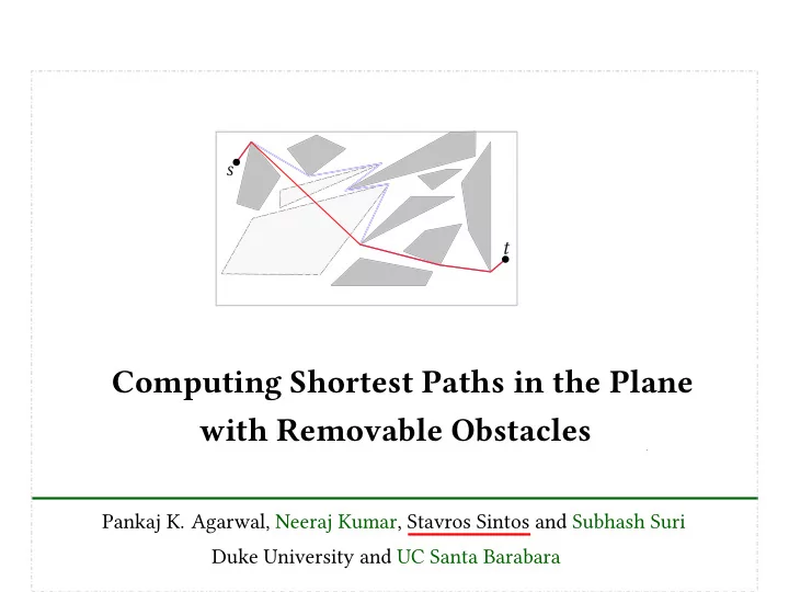
Computing Shortest Paths in the Plane
Pankaj K. Agarwal, Neeraj Kumar, Stavros Sintos and Subhash Suri
with Removable Obstacles
s t Duke University and UC Santa Barabara
SLIDE 2
s t
Problem Description
Input: h polygonal obstacles with n vertices, source s and target t
SLIDE 3
s t
Problem Description
Input: h polygonal obstacles with n vertices, source s and target t An obstacle Pi can be removed by paying cost ci
SLIDE 4
s t
Problem Description
Input: h polygonal obstacles with n vertices, source s and target t An obstacle Pi can be removed by paying cost ci Assumption: Obstacles are mutually disjoint and convex
SLIDE 5
s t
Problem Description
Input: h polygonal obstacles with n vertices, source s and target t Given a cost budget C, which obstacles should we remove An obstacle Pi can be removed by paying cost ci so that length of path from s to t is minimized? Assumption: Obstacles are mutually disjoint and convex
SLIDE 6 Motivation
Classically, we deal with finding shortest path in a fixed network
5/17
SLIDE 7 Motivation
Classically, we deal with finding shortest path in a fixed network But what if shortest paths are not good enough!
5/17
SLIDE 8 Motivation
Classically, we deal with finding shortest path in a fixed network What if we are allowed to modify the environment What changes should we make?
Desire paths
But what if shortest paths are not good enough!
5/17
SLIDE 9 Motivation
Classically, we deal with finding shortest path in a fixed network What if we are allowed to modify the environment What changes should we make? Applications But what if shortest paths are not good enough! Urban Planning Adding ‘shortcuts” to ease congestion
5/17
SLIDE 10 Motivation
Classically, we deal with finding shortest path in a fixed network What if we are allowed to modify the environment What changes should we make? Applications Reconfiguring road networks – such as by adding flyovers But what if shortest paths are not good enough!
5/17
SLIDE 11 Motivation
Classically, we deal with finding shortest path in a fixed network What if we are allowed to modify the environment What changes should we make? Applications Re-organize Warehouse Layout – Shorten frequent paths for robot But what if shortest paths are not good enough!
5/17
SLIDE 12 Path Planning Under Uncertainity
Obstacle Pi is present in input with independent probability βi, not present with probability (1 − βi)
Probability of existence = βi
SLIDE 13 Path Planning Under Uncertainity
Obstacle Pi is present in input with independent probability βi, not present with probability (1 − βi)
Probability of existence = βi
π1 π2 Path π1 has probability 1 Path π2 has probability (1 − βi)
SLIDE 14 Path Planning Under Uncertainity
Obstacle Pi is present in input with independent probability βi, not present with probability (1 − βi)
Probability of existence = βi
π1 π2 Path π1 has probability 1 Path π2 has probability (1 − βi) What is the shortest s–t path that has probability at least β?
SLIDE 15 Path Planning Under Uncertainity
Obstacle Pi is present in input with independent probability βi, not present with probability (1 − βi)
Probability of existence = βi
π1 π2 Path π1 has probability 1 Path π2 has probability (1 − βi) What is the shortest s–t path that has probability at least β? What is the most likely s–t path with length at most L?
(one that has highest probability)
SLIDE 16 Path Planning Under Uncertainity
Obstacle Pi is present in input with independent probability βi, not present with probability (1 − βi)
Probability of existence = βi
π1 π2 Path π1 has probability 1 Path π2 has probability (1 − βi) What is the shortest s–t path that has probability at least β? What is the most likely s–t path with length at most L?
(one that has highest probability)
Can reduce to the earlier cost-based model by taking negative logarithms
SLIDE 17
Related Work
Computes shortest s–t path in the plane that removes at most k obstacles O(k2n logn) algorithm using Continuous Dijkstra [HKS’17] Shortest Paths in the Plane with Obstacle Violations
SLIDE 18
Related Work
Computes shortest s–t path in the plane that removes at most k obstacles O(k2n logn) algorithm using Continuous Dijkstra [HKS’17] Shortest Paths in the Plane with Obstacle Violations Cardinality Model Obstacles have unit cost of removal, budget = k
SLIDE 19
Related Work
Computes shortest s–t path in the plane that removes at most k obstacles O(k2n logn) algorithm using Continuous Dijkstra [HKS’17] Shortest Paths in the Plane with Obstacle Violations Cardinality Model Obstacles have unit cost of removal, budget = k We study the more general cost-based model of obstacle removal
SLIDE 20 Our Results
Problem of computing a path of length at most L and cost at most C is
NP-HARD even for vertical segment obstacles.
SLIDE 21 Our Results
Problem of computing a path of length at most L and cost at most C is
NP-HARD even for vertical segment obstacles.
An FPTAS inspired from [HKS’17] running in worst case ˜
O(n2h/ϵ) time
Minimum Path length with cost at most (1 + ϵ)C
SLIDE 22 Our Results
Problem of computing a path of length at most L and cost at most C is
NP-HARD even for vertical segment obstacles.
An FPTAS inspired from [HKS’17] running in worst case ˜
O(n2h/ϵ) time
A faster FPTAS running in worst case ˜
O(nh/ϵ2) time
Minimum Path length with cost at most (1 + ϵ)C Length (1 + ϵ) times optimal, cost at most (1 + ϵ)C
SLIDE 23 Our Results
Problem of computing a path of length at most L and cost at most C is
NP-HARD even for vertical segment obstacles.
An FPTAS inspired from [HKS’17] running in worst case ˜
O(n2h/ϵ) time
A faster FPTAS running in worst case ˜
O(nh/ϵ2) time
Minimum Path length with cost at most (1 + ϵ)C Length (1 + ϵ) times optimal, cost at most (1 + ϵ)C
Data structures for fixed source approximate shortest path queries in
O(log2 n/ϵ) time, two-point queries in O(log2 n/ϵ2) time
SLIDE 24 Our Results
Problem of computing a path of length at most L and cost at most C is
NP-HARD even for vertical segment obstacles.
An FPTAS inspired from [HKS’17] running in worst case ˜
O(n2h/ϵ) time
A faster FPTAS running in worst case ˜
O(nh/ϵ2) time
Minimum Path length with cost at most (1 + ϵ)C Length (1 + ϵ) times optimal, cost at most (1 + ϵ)C
Data structures for fixed source approximate shortest path queries in
O(log2 n/ϵ) time, two-point queries in O(log2 n/ϵ2) time
Simple reduction from Partition
SLIDE 25 Our Results
Problem of computing a path of length at most L and cost at most C is
NP-HARD even for vertical segment obstacles.
An FPTAS inspired from [HKS’17] running in worst case ˜
O(n2h/ϵ) time
A faster FPTAS running in worst case ˜
O(nh/ϵ2) time
Minimum Path length with cost at most (1 + ϵ)C Length (1 + ϵ) times optimal, cost at most (1 + ϵ)C
Data structures for fixed source approximate shortest path queries in
O(log2 n/ϵ) time, two-point queries in O(log2 n/ϵ2) time
Simple reduction from Partition
Rest of the talk
SLIDE 26
A Simple FPTAS
s t Observations
SLIDE 27 A Simple FPTAS
s t Observations
The desired path π must ‘cross’ all the obstacles that were removed Since π has minimum length, it must only turn at obstacle vertices
SLIDE 28 A Simple FPTAS
s t Observations
The desired path π must ‘cross’ all the obstacles that were removed Since π has minimum length, it must only turn at obstacle vertices
Define cost(π) = sum of costs of all obstacles crossed
SLIDE 29 A Simple FPTAS
s t Observations
The desired path π must ‘cross’ all the obstacles that were removed Since π has minimum length, it must only turn at obstacle vertices
Define cost(π) = sum of costs of all obstacles crossed What is the shortest s–t path that has cost at most C?
SLIDE 30 A Simple FPTAS
Scale all costs such that budget C = h, the number of obstacles
9/17
SLIDE 31 A Simple FPTAS
Scale all costs such that budget C = h, the number of obstacles Model as a graph problem: – Nodes : s, t, obstacle vertices
9/17
SLIDE 32 A Simple FPTAS
Scale all costs such that budget C = h, the number of obstacles Model as a graph problem: – Nodes : s, t, obstacle vertices – Edges : between any pair of vertices (u,v) such that cost(uv) is at most C
c1
9/17
c2 c3
Cost of red edge is c1 + c2 + c3
SLIDE 33 A Simple FPTAS
Scale all costs such that budget C = h, the number of obstacles Model as a graph problem: – Nodes : s, t, obstacle vertices – Edges : between any pair of vertices (u,v) such that cost(uv) is at most C An edge e has two parameters: Euclidean length ℓe and cost of the edge ce
c1
9/17
c2 c3
SLIDE 34 A Simple FPTAS
Scale all costs such that budget C = h, the number of obstacles Model as a graph problem: – Nodes : s, t, obstacle vertices – Edges : between any pair of vertices (u,v) such that cost(uv) is at most C An edge e has two parameters: Euclidean length ℓe and cost of the edge ce
c1
Mimics the notion of visibility graphs, we call it a viability graph
9/17
c2 c3
SLIDE 35 A Simple FPTAS
Scale all costs such that budget C = h, the number of obstacles Model as a graph problem: – Nodes : s, t, obstacle vertices – Edges : between any pair of vertices (u,v) such that cost(uv) is at most C An edge e has two parameters: Euclidean length ℓe and cost of the edge ce Find shortest s–t path in this graph such that the cost of the path is at most C
c1
Mimics the notion of visibility graphs, we call it a viability graph
9/17
c2 c3
SLIDE 36 A Simple FPTAS
Scale all costs such that budget C = h, the number of obstacles Model as a graph problem: – Nodes : s, t, obstacle vertices – Edges : between any pair of vertices (u,v) such that cost(uv) is at most C An edge e has two parameters: Euclidean length ℓe and cost of the edge ce Find shortest s–t path in this graph such that the cost of the path is at most C
c1
Mimics the notion of visibility graphs, we call it a viability graph
(1 + ϵ)-approximation using Dijkstra’s algorithm in ˜ O( n2h ϵ ) time by creating O( h ϵ ) copies of vertices and edges
9/17
c2 c3
SLIDE 37
A Faster FPTAS
Key idea is to construct a sparse Viability Graph
SLIDE 38
A Faster FPTAS
Key idea is to construct a sparse Viability Graph Roadmap – trade a factor (1 + ϵ) in path length for efficiency
SLIDE 39
A Faster FPTAS
Key idea is to construct a sparse Viability Graph Roadmap – Construct an O(n logn) size viability graph VG1 preserving L1 distances – trade a factor (1 + ϵ) in path length for efficiency
SLIDE 40
A Faster FPTAS
Key idea is to construct a sparse Viability Graph Roadmap – Construct an O(n logn) size viability graph VG1 preserving L1 distances – Create O( 1
ϵ ) copies of VG1, one per direction and combine them to obtain VGϵ
– trade a factor (1 + ϵ) in path length for efficiency
Preserves pairwise distances within a factor of (1 + ϵ)
SLIDE 41
A Faster FPTAS
Key idea is to construct a sparse Viability Graph Roadmap – Construct an O(n logn) size viability graph VG1 preserving L1 distances – Create O( 1
ϵ ) copies of VG1, one per direction and combine them to obtain VGϵ
– trade a factor (1 + ϵ) in path length for efficiency
Preserves pairwise distances within a factor of (1 + ϵ)
– Run the modified Dijkstra on O(n
ϵ logn) size viability graph VGϵ
SLIDE 42
A Faster FPTAS
Key idea is to construct a sparse Viability Graph Roadmap – Construct an O(n logn) size viability graph VG1 preserving L1 distances – Create O( 1
ϵ ) copies of VG1, one per direction and combine them to obtain VGϵ
– trade a factor (1 + ϵ) in path length for efficiency
Preserves pairwise distances within a factor of (1 + ϵ)
– Run the modified Dijkstra on O(n
ϵ logn) size viability graph VGϵ
Primary challenge is to construct the graph VG1
SLIDE 43
A Sparse Viability Graph
Inspiration: L1 Visibility Graphs : [Clarkson-Kapoor-Vaidya’87]
SLIDE 44 A Sparse Viability Graph
Inspiration: L1 Visibility Graphs : [Clarkson-Kapoor-Vaidya’87] Main Idea: u
Do not need all O(n) edges adjacent to u
SLIDE 45 A Sparse Viability Graph
Inspiration: L1 Visibility Graphs : [Clarkson-Kapoor-Vaidya’87] Main Idea: u v
Do not need all O(n) edges adjacent to u
SLIDE 46 A Sparse Viability Graph
Inspiration: L1 Visibility Graphs : [Clarkson-Kapoor-Vaidya’87] Main Idea: u v
Do not need all O(n) edges adjacent to u Take projections on a ‘split line’ ℓ
SLIDE 47 A Sparse Viability Graph
Inspiration: L1 Visibility Graphs : [Clarkson-Kapoor-Vaidya’87] Main Idea: u v
Do not need all O(n) edges adjacent to u Take projections on a ‘split line’ ℓ
SLIDE 48 A Sparse Viability Graph
Inspiration: L1 Visibility Graphs : [Clarkson-Kapoor-Vaidya’87] Main Idea: u v
Do not need all O(n) edges adjacent to u Take projections on a ‘split line’ ℓ
u v
SLIDE 49 Also need at most four projections on neighboring obstacles
A Sparse Viability Graph
Inspiration: L1 Visibility Graphs : [Clarkson-Kapoor-Vaidya’87] Main Idea: u v
Do not need all O(n) edges adjacent to u Take projections on a ‘split line’ ℓ
u v Total size: O(n logn)
SLIDE 50 Also need at most four projections on neighboring obstacles
A Sparse Viability Graph
Inspiration: L1 Visibility Graphs : [Clarkson-Kapoor-Vaidya’87] Main Idea: u v
Do not need all O(n) edges adjacent to u Take projections on a ‘split line’ ℓ
u v Total size: O(n logn) We show how to construct O(n logn) size L1 Viability Graphs
edges can go through obstacles
SLIDE 51 Algorithm Overview
Will reuse idea of taking split line projections for [CKV’87]
SLIDE 52 Algorithm Overview
Will reuse idea of taking split line projections for [CKV’87]
can be naturally extended to edges of viability graph
SLIDE 53 Algorithm Overview
Will reuse idea of taking split line projections for [CKV’87]
can be naturally extended to edges of viability graph However, taking projections on four neighboring obstacles is not sufficient
SLIDE 54 Algorithm Overview
Will reuse idea of taking split line projections for [CKV’87]
can be naturally extended to edges of viability graph However, taking projections on four neighboring obstacles is not sufficient We circumvent this problem by adding “bypass vertices” Using this model we give an arguably simpler proof
- f correctness for the more general viability graphs
SLIDE 55 Algorithm Overview
Will reuse idea of taking split line projections for [CKV’87]
can be naturally extended to edges of viability graph However, taking projections on four neighboring obstacles is not sufficient We circumvent this problem by adding “bypass vertices” Using this model we give an arguably simpler proof
- f correctness for the more general viability graphs
Next we describe an algorithm for constructing an L1 viability graph VG1
SLIDE 56
Obstacles with Costs ⇒ Segments with Costs
SLIDE 57
Obstacles with Costs ⇒ Segments with Costs
π1 π2 Obstacles are convex and disjoint ⇒ Shortest paths intersect zero or exactly two sides of an obstacle
SLIDE 58
Obstacles with Costs ⇒ Segments with Costs
π1 π2 Obstacles are convex and disjoint ⇒ Shortest paths intersect zero or exactly two sides of an obstacle Assign cost ci/2 to all segments of an obstacle that has cost ci
SLIDE 59
Obstacles with Costs ⇒ Segments with Costs
π1 π2 Obstacles are convex and disjoint ⇒ Shortest paths intersect zero or exactly two sides of an obstacle Assign cost ci/2 to all segments of an obstacle that has cost ci Allows us to reason about geometry of line segments
SLIDE 60
Algorithm Description
v w
SLIDE 61 Algorithm Description
v w ℓ
Find the split line ℓ that splits vertices into equal sized sets Vl and Vr
SLIDE 62 Algorithm Description
v w ℓ v′ w′
Find the split line ℓ that splits vertices into equal sized sets Vl and Vr Let v′ be the projection of v on this split line ℓ
– Add vertex v′ and edge vv′ with cost c(vv′) – Cost of projection segment is the sum of
costs of all obstacle segments that it intersects
SLIDE 63 Algorithm Description
v w ℓ w2 v′ w′ v1 w1 v2
Find the split line ℓ that splits vertices into equal sized sets Vl and Vr Let v′ be the projection of v on this split line ℓ
– Add vertex v′ and edge vv′ with cost c(vv′)
Find first segment s′ of positive slope that intersects ℓ
– Add two bypass vertices v1,v2 and edges vv′ and v1v2 – Bypass edges v1v2 have cost c(v1v2) = 0 – Cost of projection segment is the sum of
costs of all obstacle segments that it intersects
SLIDE 64 Algorithm Description
v w ℓ w2 v′ w′ v1 w1 v2
Find the split line ℓ that splits vertices into equal sized sets Vl and Vr Let v′ be the projection of v on this split line ℓ
– Add vertex v′ and edge vv′ with cost c(vv′)
Find first segment s′ of positive slope that intersects ℓ
– Add two bypass vertices v1,v2 and edges vv′ and v1v2
Connect consecutive vertices on ℓ and obstacle boundary
SLIDE 65 Algorithm Description
v w ℓ w2 v′ w′ ℓ v w v1 w1 v2
Find the split line ℓ that splits vertices into equal sized sets Vl and Vr Let v′ be the projection of v on this split line ℓ
– Add vertex v′ and edge vv′ with cost c(vv′)
Find first segment s′ of positive slope that intersects ℓ
– Add two bypass vertices v1,v2 and edges vv′ and v1v2
Connect consecutive vertices on ℓ and obstacle boundary Repeat for a horizontal split line. Recurse on sets Vl and Vr .
SLIDE 66
Correctness
Suffices to show: for any pair of obstacle vertices p,q there exists a path πpq such that the L1 length ∥πpq∥1 ≤ ∥pq∥1 and cost c(πpq) ≤ c(pq) Proof Idea:
SLIDE 67
Correctness
Suffices to show: for any pair of obstacle vertices p,q there exists a path πpq such that the L1 length ∥πpq∥1 ≤ ∥pq∥1 and cost c(πpq) ≤ c(pq) Proof Idea: p q
SLIDE 68
Correctness
Suffices to show: for any pair of obstacle vertices p,q there exists a path πpq such that the L1 length ∥πpq∥1 ≤ ∥pq∥1 and cost c(πpq) ≤ c(pq) Proof Idea: p sy sx Define a region (clipped rectangle) Rpq q
SLIDE 69
Correctness
Suffices to show: for any pair of obstacle vertices p,q there exists a path πpq such that the L1 length ∥πpq∥1 ≤ ∥pq∥1 and cost c(πpq) ≤ c(pq) Proof Idea: p sy sx Define a region (clipped rectangle) Rpq q Proof by induction on number of vertices in Rpq – If Rpq contains an obstacle vertex – If Rpq does not contains an obstacle vertex
SLIDE 70
Correctness
Suffices to show: for any pair of obstacle vertices p,q there exists a path πpq such that the L1 length ∥πpq∥1 ≤ ∥pq∥1 and cost c(πpq) ≤ c(pq) Proof Idea: p sy sx Define a region (clipped rectangle) Rpq q Proof by induction on number of vertices in Rpq – If Rpq contains an obstacle vertex – If Rpq does not contains an obstacle vertex (Induction Step) (Base Case)
SLIDE 71
Induction Step
p q lr r
SLIDE 72
Induction Step
p q lr r We show how to find an intermediate vertex r such that
SLIDE 73
Induction Step
p q lr r We show how to find an intermediate vertex r such that such that ∥pr∥1 + ∥rq∥1 ≤ ∥pq∥1 and cost c(pr) + c(rq) ≤ c(pq)
SLIDE 74
Induction Step
p q lr r We show how to find an intermediate vertex r such that such that ∥pr∥1 + ∥rq∥1 ≤ ∥pq∥1 and cost c(pr) + c(rq) ≤ c(pq) Details are technical, relies heavily on disjointness of obstacle segments
SLIDE 75
Base Case
ℓ B C Identify three types of edges A, B and C p A q
SLIDE 76
Base Case
ℓ B C Identify three types of edges A, B and C Identify three types of edges A, B and C – Type B and C edges cannot co-exist p A q
SLIDE 77
Base Case
ℓ B C Identify three types of edges A, B and C Identify three types of edges A, B and C – Type B and C edges cannot co-exist Type B edge + vertical split line ≡ Type C edge + horizontal split line p A q
SLIDE 78
Base Case
ℓ B Identify three types of edges A, B and C Identify three types of edges A, B and C – Type B and C edges cannot co-exist Type B edge + vertical split line ≡ Type C edge + horizontal split line Exists a path πpq in VG1 using projection and bypass vertices p A q
SLIDE 79
Base Case
ℓ B Identify three types of edges A, B and C Identify three types of edges A, B and C – Type B and C edges cannot co-exist Type B edge + vertical split line ≡ Type C edge + horizontal split line Exists a path πpq in VG1 using projection and bypass vertices Easy to verify that πpq has same L1 length and cost as the segment pq p A q
SLIDE 80
A Faster FPTAS
Key idea is to construct a sparse Viability Graph Roadmap – Construct an O(n logn) size viability graph VG1 preserving L1 distances – Create 1/ϵ copies of VG1, one per direction and combine them to obtain VGϵ – trade a factor (1 + ϵ) in path length for efficiency
Preserves pairwise distances within a factor of (1 + ϵ)
– Run the slower FPTAS on O(n
ϵ logn) size viability graph VGϵ
Primary challenge is to construct the graph VG1
SLIDE 81
A Faster FPTAS
Key idea is to construct a sparse Viability Graph Roadmap – Construct an O(n logn) size viability graph VG1 preserving L1 distances – Create 1/ϵ copies of VG1, one per direction and combine them to obtain VGϵ – trade a factor (1 + ϵ) in path length for efficiency
Preserves pairwise distances within a factor of (1 + ϵ)
– Run the slower FPTAS on O(n
ϵ logn) size viability graph VGϵ
Primary challenge is to construct the graph VG1
✓
SLIDE 82
In Summary
SLIDE 83 In Summary
Motivated by applications, we study the problem of computing shortest
path among removable obstacles
SLIDE 84 In Summary
Motivated by applications, we study the problem of computing shortest
path among removable obstacles
We show that computing such a path exactly is NP-hard.
SLIDE 85 In Summary
Motivated by applications, we study the problem of computing shortest
path among removable obstacles
We show that computing such a path exactly is NP-hard. A simple (1 + ϵ)-approximation follows using the idea of viability
graphs (an extension of visibility graphs)
SLIDE 86 In Summary
Motivated by applications, we study the problem of computing shortest
path among removable obstacles
We show that computing such a path exactly is NP-hard. A simple (1 + ϵ)-approximation follows using the idea of viability
graphs (an extension of visibility graphs)
Obtain a faster approximation by constructing a sparse viability graph
SLIDE 87 In Summary
Motivated by applications, we study the problem of computing shortest
path among removable obstacles
We show that computing such a path exactly is NP-hard. A simple (1 + ϵ)-approximation follows using the idea of viability
graphs (an extension of visibility graphs)
Obtain a faster approximation by constructing a sparse viability graph Obtained data structures for approximate shortest path queries running
in polylogarithmic time
SLIDE 88 In Summary
Motivated by applications, we study the problem of computing shortest
path among removable obstacles
We show that computing such a path exactly is NP-hard. A simple (1 + ϵ)-approximation follows using the idea of viability
graphs (an extension of visibility graphs)
Obtain a faster approximation by constructing a sparse viability graph Obtained data structures for approximate shortest path queries running
in polylogarithmic time
Applied these results to solve a shortest path problem in a stochastic
model of obstacles
SLIDE 89 In Summary
Motivated by applications, we study the problem of computing shortest
path among removable obstacles
We show that computing such a path exactly is NP-hard. A simple (1 + ϵ)-approximation follows using the idea of viability
graphs (an extension of visibility graphs)
Obtain a faster approximation by constructing a sparse viability graph Obtained data structures for approximate shortest path queries running
in polylogarithmic time
Applied these results to solve a shortest path problem in a stochastic
model of obstacles
Thanks!
SLIDE 90
Backup : NP-Hardness
Simple reduction from Partition ai t Gi a1 an . . . . . . s A is a set of integers, ai corresponds to group Gi
SLIDE 91 Backup : NP-Hardness
Simple reduction from Partition ai t Gi a1 an . . . . . . s A is a set of integers, ai corresponds to group Gi
Go through the middle obstacle by paying cost ai Go around it by adding a detour of length ai
Path must go through the channel
SLIDE 92 Backup : NP-Hardness
Simple reduction from Partition ai t Gi a1 an . . . . . . s A is a set of integers, ai corresponds to group Gi
Go through the middle obstacle by paying cost ai Go around it by adding a detour of length ai
An s–t path with length at most L = 1
2 ∑ai and cost at most C = 1 2 ∑ai exists
Path must go through the channel
if and only if set A can be partitioned into two equal groups.