Codes, matroids and trellises occur at several levels. Do you (a) - - PDF document

SLIDE 1

Codes, matroids and trellises

Peter J Cameron

(with many contributions from C. Papadopoulos,

• R. A. Bailey and C. G. Rutherford)

School of Mathematical Sciences Queen Mary and Westfield College London E1 4NS p.j.cameron@qmw.ac.uk Combinatorics 2000, Gaeta

1

Who discovered the Hamming codes?

Was it

• R. W. Hamming?
• M. J. E. Golay?
• R. A. Fisher?
• J. J. Sylvester?

See “Hamming and Golay, Fisher and Bose” on this Web page for more about this.

2

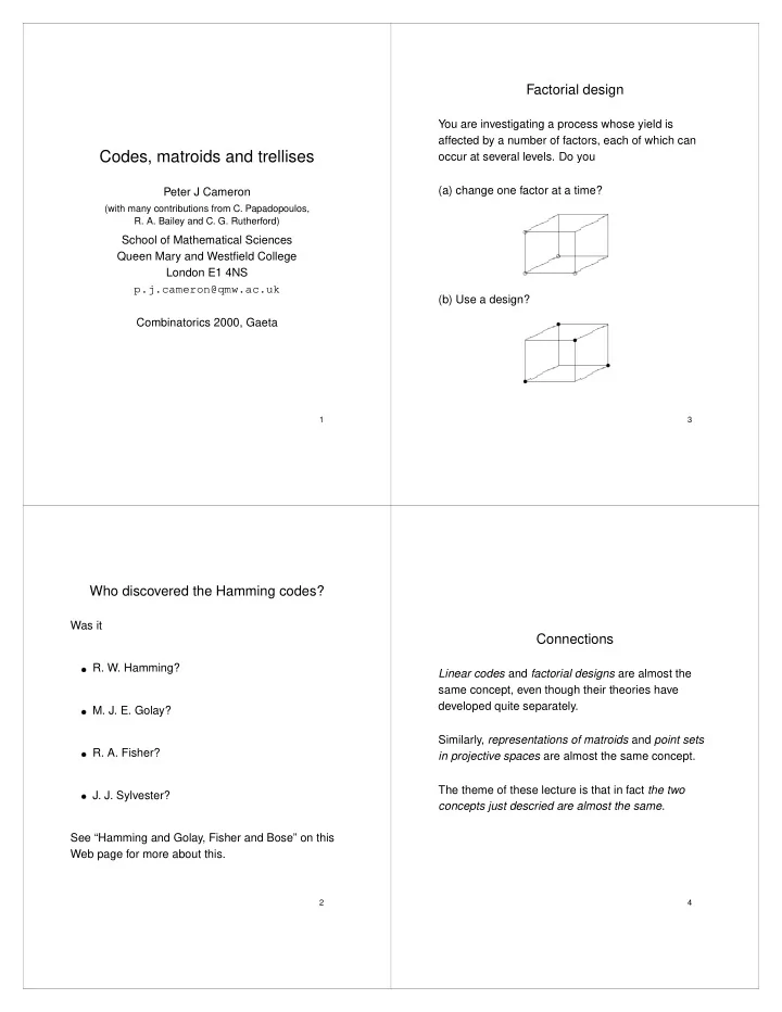
Factorial design

You are investigating a process whose yield is affected by a number of factors, each of which can

• ccur at several levels. Do you

(a) change one factor at a time?

✁ ✁ ✁ ✁ ✁ ✁ ✁ ✁ ✁ ✁ ✁ ✁ ✁ ✁ ✁ ✁ ✁ ✁ ✁ ✁ ✁ ✁ ✁ ✁ ✂ ✂ ✂ ✂

(b) Use a design?

✁ ✁ ✁ ✁ ✁ ✁ ✁ ✁ ✁ ✁ ✁ ✁ ✁ ✁ ✁ ✁ ✁ ✁ ✁ ✁ ✁ ✁ ✁ ✁ ✄ ✄ ✄ ✄

3

Connections

Linear codes and factorial designs are almost the same concept, even though their theories have developed quite separately. Similarly, representations of matroids and point sets in projective spaces are almost the same concept. The theme of these lecture is that in fact the two concepts just descried are almost the same.

4

SLIDE 2

Codes

A linear code C of length n and dimension k over a field F is a k-dimensional subspace of Fn. The weight wt

☎ v ✆ of a word v ✝

Fn is the number of non-zero coordinates, and the minimum weight of C is the smallest weight of a non-zero vector in C. Codes C and C

✞ are monomial equivalent if C ✞ is

• btained from C by permuting the coordinates and

multiplying them by non-zero scalars. Theorem 1 A code with minimum weight d can correct up to

✟ ☎ d ✠

1

✆☛✡ 2 ☞ errors.

5

Matroids

A matroid M on a set E is a family

✌

• f subsets of E

called independent sets, closed under taking subsets and satisfying the exchange property. The rank ρ

☎ A ✆ of a subset A of E is the size of the

largest independent subset of A. An independent subset of E of size ρ

☎ E ✆ is called a basis of M.

• Example. The uniform matroid U

☎ k ✍ n ✆ : the

independent sets are all subsets having cardinality at most k. A representation of E over a field F is a map of E into an F-vector space which preserves independence. Two representations are equivalent if they are related by an invertible linear transformation between the vector spaces.

6

Exchange axiom

The exchange axiom states: If A and B are independent sets such that

✎ B ✎✑✏✒✎ A ✎ , then there exists

b

✝

B

✓ A such that A ✔✖✕ b ✗ is independent.

This guarantees that all bases have the same cardinality, and so makes the definition of rank sensible.

7

The code-matroid connection

Let A be a k

✘ n matrix over a field F having rank k.

From A we construct

• a code C

☎ A ✆ generated by the rows of A;

• a matroid M

☎ A ✆ represented in Fk by the columns

• f A.

The equivalence relation on such matrices given by arbitary row operations and monomial column

• perations mirrors the natural notions of equivalence

for linear codes and representations of matroids. Note to geometers: Linear MDS codes in projective space over GF

☎ q ✆ correspond to representations of

the uniform matroid U

☎ n ✍ k ✆ over GF ☎ q ✆ .

8

SLIDE 3

First and last base

Let the ground set E of the matroid M be totally

• rdered, and let ρ

☎ E ✆✚✙

• k. Let

✛

be the set of bases

• f M. When we write a base as

✕ b1 ✍☛✜✢✜☛✜☛✍ bk ✗ , we

assume that b1

✣✥✤☛✤☛✤✦✣

bk. The (lexicographically) first base F

✙✒✕ f1 ✍☛✜☛✜☛✜✢✍ fk ✗

satisfies fi

✧

bi for any base B

✙✒✕ b1 ✍☛✜☛✜✢✜☛✍ bk ✗ .

Dually the last base L

✙★✕ l1 ✍☛✜☛✜✢✜☛✍ lk ✗ satisfies bi ✧

li for any base B

✙✒✕ b1 ✍☛✜☛✜☛✜✢✍ bk ✗ .

These properties express the relationship of matroids to the greedy algorithm.

9

Weight enumerator and Tutte polynomial

The weight enumerator of a code C of length n is given by WC

☎ x ✍ y ✆✩✙

∑

c

✪ C

xn

✫ wt ✬ c ✭ ywt ✬ c ✭ ✜

The Tutte polynomial of a matroid M on E with rank function ρ is given by T

☎ M;x ✍ y ✆✩✙

∑

A

✮ E ☎ x ✠

1

✆ ρE ✫ ρA ☎ y ✠

1

✆✰✯ A ✯ ✫ ρA ✜

10

Internal and external activity

There is an equivalent definition as follows. Suppose that M is a matroid on the set E, which is totally

• rdered. Let B be a base of M. An element b

✝

B is internally active with respect to B if, for all c

✝

B, we have B

✔✱✕ c ✗✚✓✲✕ b ✗✳✝✖✛✵✴

c

✣

• b. The internal activity of

a base is the number of internally active elements associated with it. Dually, an element e

✡ ✝

B is externally active with respect to B if, for all f

✝

B, we have f

✝ C ☎ e ✍ B ✆✚✴

f

✣

e.The external activity of a base is the number of externally active elements associated with it. Then we have T

☎ M;x ✍ y ✆✩✙

∑

B

✪✷✶

ti

✸ jxiyi

where ti

✸ j is the number of bases with i internally

active elements and j externally active elements.

11

First and last; internal and external

A loop in a matroid is an element e

✝

E which is contained in no basis. A coloop is an element e

✝

E which is contained in every basis. Note that (a) The internal activity of the first base is the number of coloops of M, while its external activity is equal to

✎ E ✎✹✠

ρ

☎ E ✆ .

(b) The internal activity of the last base is ρ

☎ E ✆ ,

while its external activity is equal to the number

• f loops of M.

12

SLIDE 4

Greene’s Theorem

Curtis Greene showed in 1975 that the weight enumerator of C

✙

C

☎ A ✆ is a specialisation of the

Tutte polynomial of M

✙

M

☎ A ✆ :

Theorem 2 WC

☎ x ✍ y ✆✩✙

yn

✫ dim ✬ C ✭ ☎ x ✠

y

✆ dim ✬ C ✭ T ✺

M; x

✻ ☎ q ✠

1

✆ y

x

✠

y

✍ x

y

✼ ✜

In particular, the Tutte polynomial of M

☎ A ✆ determines

the minimum weight of C

☎ A ✆ .

13

Duality

The dual of a matroid M on E is the matroid M

✽ on E

whose bases are the complements of the bases of M. The dual of a code C is the code C

✾✿✙✒✕ v ✝

Fn : v

✤ c ✙

0 for all c

✝ C ✗❀✍

where

✤ is the usual dot product.

Under the code–matroid connection, dual codes correspond to dual matroids. Also, it is trivial that T

☎ M ✽ ;x ✍ y ✆✩✙

T

☎ M;y ✍ x ✆❁✍

from which we obtain the MacWilliams relation WC

❂ ☎ x ✍ y ✆❃✙

1

✎C ✎ WC ☎ x ✻ ☎ q ✠

1

✆ y ✍ x ✠

y

✆❁✜

14

An example

Suppose that we are using the binary dual Hamming code of length 7 to send information. The codewords are: 0000000 0011011 0101101 0110110 1001110 1010101 1100011 1111000 The minimum weight is 4, so we can correct one error and detect two errors.

15

Analog errors

In practice, the received word is an analog signal, sampled at seven time points, i.e. seven real

• numbers. Suppose that we receive

w

✙ ☎ ✠ 0 ✜ 1 ✍ 0 ✜ 0 ✍ 0 ✜ 2 ✍ 0 ✜ 9 ✍ 1 ✜ 8 ✍ 0 ✜ 9 ✍ 1 ✜ 4 ✆✚✝✖❄

7

✜

If we round each value to the nearest of zero and

• ne, we obtain 0001111, which is at distance 2 from

the second, third and fifth codewords in the list, so we have a decoding failure. If we make the (physically realistic) assumptions that the errors at the sampling points are independent identically distributed Gaussian variables, then it can be shown that the most likely codeword to have been transmitted is the one at smallest Euclidean distance from w in

❄

7, which turns out to be 0101101.

16

SLIDE 5

A trellis

A trellis for the dual Hamming code:

❅✢❆ ❇✢❈

A

❅✢❆ ❇✢❈

C

❅✢❆ ❇✢❈

B

❅✢❆ ❇✢❈

G

❅✢❆ ❇✢❈

F

❅✢❆ ❇✢❈

E

❅✢❆ ❇✢❈

D

❅✢❆ ❇✢❈

Z

❅✢❆ ❇✢❈

H

❅✢❆ ❇✢❈

I

❅✢❆ ❇✢❈

J

❅✢❆ ❇✢❈

K

❅✢❆ ❇✢❈

L

❅✢❆ ❇✢❈

M

❅✢❆ ❇✢❈

N

❅✢❆ ❇✢❈

O

❅✢❆ ❇✢❈

P

❅✢❆ ❇✢❈

Q

❅✢❆ ❇✢❈

R

❅✢❆ ❇✢❈

S

❅✢❆ ❇✢❈

T

❅✢❆ ❇✢❈

U

❅✢❆ ❇✢❈

V

❅✢❆ ❇✢❈

W

❅✢❆ ❇✢❈

X

❅✢❆ ❇✢❈

Y

❉ ❉ ❉ ❉ ❉

1

❊ ❊ ❊ ❊ ❊ ❋ ❋ ❋ ❋ ❋ ❋ ❋

1

• 1

❉ ❉ ❉ ❉ ❉ ❉ ❉ ❉ ❉ ❉ ❉ ❉ ❉ ❉ ❉ ❉ ❉ ❉ ❉ ❉

1 1 1 1

❊ ❊ ❊ ❊ ❊

1

• ❍

❍ ❍ ❍ ❍ ❍ ❍ ❍ ❍ ❍ ❍ ■ ■ ■ ■ ■ ■ ■ ■ ■ ■ ■ ■ ■ ■ ■

1

❏ ❏ ❏ ❏ ❏ ❏ ❏ ❏ ❏ ❏ ❏ ❋ ❋ ❋ ❋ ❋ ❋ ❋

1

❉ ❉ ❉ ❉ ❉

1

• 1

❋ ❋ ❋ ❋ ❋ ❋ ❋

1

• 1

❋ ❋ ❋ ❋ ❋ ❋ ❋

1

❋ ❋ ❋ ❋ ❋ ❋ ❋ ❊ ❊ ❊ ❊ ❊ ❉ ❉ ❉ ❉ ❉

1 The codewords are the sequences of labels on the paths from A to Z.

17

Trellis decoding

❅✢❆ ❇✢❈

A

❑ 00 ❅✢❆ ❇✢❈

C

❑ 01 ❅✢❆ ❇✢❈

B

1

❑ 21 ❅✢❆ ❇✢❈

G

1

❑ 01 ❅✢❆ ❇✢❈

F

❑ 01 ❅✢❆ ❇✢❈

E

1

❑ 21 ❅✢❆ ❇✢❈

D

2

❑ 21 ❅✢❆ ❇✢❈

Z

2

❑ 67 ❅✢❆ ❇✢❈

H

2

❑ 75 ❅✢❆ ❇✢❈

I

2

❑ 25 ❅✢❆ ❇✢❈

J

1

❑ 75 ❅✢❆ ❇✢❈

K

1

❑ 25 ❅✢❆ ❇✢❈

L

❑ 05 ❅✢❆ ❇✢❈

M

❑ 65 ❅✢❆ ❇✢❈

N

1

❑ 05 ❅✢❆ ❇✢❈

O

1

❑ 65 ❅✢❆ ❇✢❈

P

❑ 86 ❅✢❆ ❇✢❈

Q

❑ 66 ❅✢❆ ❇✢❈

R

1

❑ 06 ❅✢❆ ❇✢❈

S

1

❑ 26 ❅✢❆ ❇✢❈

T

4

❑ 10 ❅✢❆ ❇✢❈

U

3

❑ 90 ❅✢❆ ❇✢❈

V

1

❑ 90 ❅✢❆ ❇✢❈

W

1

❑ 70 ❅✢❆ ❇✢❈

X

1

❑ 91 ❅✢❆ ❇✢❈

Y

2

❑ 51 ❉ ❉ ❉ ❉ ❉ ❉

1

❑ 21 ❊ ❊ ❊ ❊ ❊ ❊ ❑ 01 ❋ ❋ ❋ ❋ ❋ ❋ ❋ ❋

1

❑ 00

• 1

❑ 00 ❑ 00 ❑ 00 ❉ ❉ ❉ ❉ ❉ ❉ ❉ ❉ ❉ ❉ ❉ ❉ ❉ ❉ ❉ ❉ ❉ ❉ ❉ ❉ ❉ ❉ ❉ ❉ ❑ 64 ❑ 64 ❑ 04 ❑ 04 ❑ 04 ❑ 04 ❑ 64 ❑ 64 ❊ ❊ ❊ ❊ ❊ ❊ ❑ 01

• ❑ 81

❍ ❍ ❍ ❍ ❍ ❍ ❍ ❍ ❍ ❍ ❍ ❍0 ❑ 81 ■ ■ ■ ■ ■ ■ ■ ■ ■ ■ ■ ■ ■ ■ ■ ■ ■ ❑ 01 ❏ ❏ ❏ ❏ ❏ ❏ ❏ ❏ ❏ ❏ ❏ ❏ ❑ 81 ❋ ❋ ❋ ❋ ❋ ❋ ❋ ❋ ❑ 01 ❉ ❉ ❉ ❉ ❉ ❉ ❑ 01 ❑ 81

3

❑ 24

3

❑ 24

• ❑ 64

❋ ❋ ❋ ❋ ❋ ❋ ❋ ❋ ❑ 64

• ❑ 81
• ❑ 01

❋ ❋ ❋ ❋ ❋ ❋ ❋ ❋ ❑ 01 ❋ ❋ ❋ ❋ ❋ ❋ ❋ ❋ ❑ 81 ❊ ❊ ❊ ❊ ❊ ❊

1

❑ 96 ❉ ❉ ❉ ❉ ❉ ❉ ❑ 16

The shortest squared Euclidean distance from received word to codeword is equal to the length of the shortest path from A to Z. The shortest path is ACGNRWYZ, and the decoded word is 0101101.

18

Muder’s Theorem

The best trellis for a code will have the fewest vertices or edges, or smallest cycle rank. For a linear code, there is a trellis which is uniformly best: Theorem 3 Let C be a linear code of length n. Then there is a trellis T representing C, with layers V0

✍✢✜☛✜☛✜☛✍ Vn, such that, if another proper trellis T ✞ for C

has layers V

✞ ✍☛✜☛✜✢✜☛✍ V ✞

n, then

✎V ✞

i

✎▼▲◆✎Vi ✎ for i ✙ ✍☛✜☛✜☛✜☛✍ n.

Moreover, if

✎V ✞

i

✎❖✙P✎Vi ✎ for i ✙ ✍☛✜☛✜☛✜☛✍ n, then T ✞ is

isomorphic to T. Furthermore, T also minimises the sizes of all the edge layers and the cycle rank.

19

Past and future

For 0

✧

i

✧

n, we define the ith past subcode of C to be Pi

✙✒✕ c ✝ C : cj ✙

0 for all j

✏

i

✗❀✍

and the ith future subcode to be Fi

✙✒✕ c ✝ C : cj ✙

0 for all j

✧

i

✗❀✜

By convention, Pn

✙

F0

✙

C. If A and B denote the first and last bases for M, then dim

☎ Fi ✆◗✙❘✎ A ❙✖✕ i ✻

1

✍☛✜☛✜☛✜☛✍ n ✗❚✎ ✍

dim

☎ Pi ✆◗✙❘✎ B ❙✖✕ 1 ✍☛✜✢✜☛✜☛✍ i ✗❚✎ ✜

Let Vi

✙

C

✡ ☎ Pi ❯

Fi

✆ . For each codeword c, put an

edge with label ci from

☎ Pi ✫ 1 ❯

Fi

✫ 1 ✆❱✻

c

✝ Vi ✫ 1 to the

coset

☎ Pi ❯

Fi

✆❱✻

c

✝ Vi. Identify edges with the same

label between the same vertices. This is the Muder trellis for C.

20

SLIDE 6

Equivalent codes

Equivalent codes may have Muder trellises of different size. The problem of finding the smallest Muder trellis for a code equivalent to C is NP-complete in general. However, using the matroid allows us to produce bounds (or exact values) for many important codes. We must order so that the first base is as late as possible, and the last base as early as possible. Of course, these requirements conflict. For example, a code is MDS if and only the matroid is

• uniform. In this case, regardless of permutations, the

first base is

✕ 1 ✍☛✜☛✜☛✜✢✍ k ✗ and the last base is ✕ n ✠

k

✻

1

✍☛✜✢✜☛✜✹✍ n ✗ . So the trellis is as large as possible,

no matter how we permute coordinates.

21

Hamming weight hierarchy

The ith generalised Hamming weight of a code C is the smallest size di of the support of an i-dimensional subcode of C. So, for example, d1 is the minimum weight of C. The Hamming weight hierarchy is

☎ d1 ✍ d2 ✍☛✜☛✜☛✜✢✍ dk ✆ .

Note that it is determined by the Tutte polynomial. Bounds for di can be obtained from the Griesmer bound and other methods; for example, di

❲ 1 ▲

di

✻❨❳ di ☎ q ✠

1

✆

q

☎ qi ✠

1

✆❬❩ ✜

Theorem 4 The first and last bases of the

❭ n ✍ k ❪ code

C satisfy ai

✧

n

✠

dk

✫ i ❲ 1 ☎ C ✆❫✻

1

✍

bi

▲

di

☎ C ✆❁✜

If these bounds are attained then the Muder trellis for C is smaller than that for any equivalent code.

22

The binary Golay code

The Hamming weight hierarchy for the extended binary Golay code is

✕ 8 ✍ 12 ✍ 14 ✍ 15 ✍ 16 ✍ 18 ✍ 19 ✍ 20 ✍ 21 ✍ 22 ✍ 23 ✍ 24 ✗❀✜

The coordinates can be ordered so that this is the last base, and the first base is its complement. So the bounds of Theorem 4 are attained. Indeed, this will hold as long as we ensure that

✕✦✕ 1 ✍ 2 ✍ 3 ✍ 4 ✗❀✍✹✕ 5 ✍ 6 ✍ 7 ✍ 8 ✗❀✍☛✜✢✜☛✜❴✍✹✕ 21 ✍ 22 ✍ 23 ✍ 24 ✗✦✗

is a sextet. (Since the code is self-dual, the complement of the first base is the last base.) Hence the smallest trellis for the extended binary Golay code has 2686 vertices.

23