Clustering In this example distance matrix: and have the most - PDF document

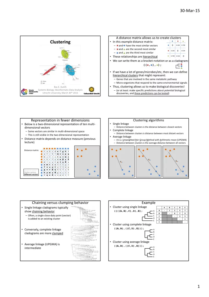
30 ‐ Mar ‐ 15 A distance matrix allows us to create clusters Clustering • In this example distance matrix: and have the most similar vectors 0 0.265 0.799 – and are the second most similar – 0.265 0 0.534 and are the third most similar – • These relationships are hierarchical 0 0.799 0.534 • We can write them as a bracket ‐ notation or as a cladogram: (( , ), ); (( , ), ); • If we have a lot of genes/microbes/etc, then we can define hierarchical clusters that might represent: – Genes that are involved in the same metabolic pathway – Micro ‐ organisms that respond to the same environmental signals • Thus, clustering allows us to make biological discoveries! Bas E. Dutilh Systems Biology: Bioinformatic Data Analysis – (or at least: make specific predictions about potential biological Utrecht University, March 30 th 2015 discoveries, and these predictions can be tested) Representation in fewer dimensions Clustering algorithms • Single linkage • Below is a two ‐ dimensional representation of ten multi ‐ – Distance between clusters is the distance between closest vectors dimensional vectors • Complete linkage – Some vectors are similar in multi ‐ dimensional space – Distance between clusters is distance between most distant vectors – This is still visible in the two ‐ dimensional representation • Average linkage • Distance matrix depends on distance measure (previous – A.k.a. Unweighted Pair Group Method with Arithmetic mean (UPGMA) lecture) – Distance between clusters is the average distance between all vectors Distance matrix: 0 0 a b a b c c d d e e f f g g h h i i a a 0 0 j j k k l l m n m n o p o p q q b b j j 0 0 r r s s t t u u v w x v w x c c k k r r 0 0 y y z α z α β γ β γ δ δ d d d d d l l s s y y 0 0 ε ε ζ ζ η θ η θ ι ι e m t e m t z z ε ε 0 0 κ κ λ μ λ μ ν ν f f n u n u α α ζ ζ κ κ 0 0 ξ ξ π π ρ ρ g g o v o v β β η η λ λ ξ ξ 0 0 ς ς σ σ Identical vector Similar vectors h h p w γ p w γ θ θ μ π μ π ς ς 0 0 τ τ Different vectors i i q q x x δ δ ι ι ν ρ ν ρ σ σ τ τ 0 0 Chaining versus clumping behavior Example • Cluster using single linkage • Single linkage cladograms typically A B C D E A ‐ 1 2 5 7 show chaining behavior ((((A,B),C),D),E); A B B ‐ 8 7 9 – Often, a single close data point (vector) C C ‐ 3 5 D is added to an existing cluster D ‐ 5 E E ‐ • Cluster using complete linkage ((A,B),((C,D),E))); • Conversely, complete linkage y, p g A B cladograms are more clumped C D E • Cluster using average linkage • Average linkage (UPGMA) is ((A,B),((C,D),E))); A intermediate B C D E 1

30 ‐ Mar ‐ 15 Branch lengths Effect of distance measures on clustering • Cluster using average linkage (UPGMA) ((A,B),((C,D),E))); A B C D E 0. 25 A ‐ 1 2 5 7 Euclidian B ‐ 8 7 9 0. 20 C ‐ 3 5 Gene 1 /Expression D ‐ 5 Gene 1 Gene 2 E ‐ 0. 15 Gene 2 Gene 3 0 5 0.5 A Abundance/ A 3.17 0. 10 B 0.5 B Gene 3 Correlation C 1.5 C 5 0.0 1 Gene 1 D 1.5 D 0.67 Gene 3 0 E 2.5 E Gene 2 1 2 3 4 5 6 7 8 9 10 Time/environments/samples… ((A ,B ) ,((C ,D ) ,E ) )); :0.5 :0.5 :3.17 :1.5 :1.5 :1 :2.5 :0.67 Changing perspective Bi ‐ clustering 0. 25 Between the genes (etc) 0. 20 0 x y Abundance/Expression 0. 15 x 0 z 0. 10 y z 0 0.0 5 1 1 2 3 2 3 4 4 5 6 7 5 6 7 8 9 10 8 9 10 Genes 0 Between the samples (etc) 1 0 a b c d e f g h i 1 2 3 4 5 6 7 8 9 10 2 a 0 j k l m n o p q Time/Environments/Samples 3 b j 0 r s t u v w x 4 c k r 0 y z α β γ δ 1 0.20 0.15 0.12 2 0.17 0.15 0.09 5 d l s y 0 ε ζ η θ ι 3 0.16 0.16 0.08 6 e m t z ε 0 κ λ μ ν 4 0.20 0.15 0.11 7 f n u α ζ κ 0 ξ π ρ 5 0.20 0.16 0.12 6 0.17 0.16 0.10 8 g o v β η λ ξ 0 ς σ 7 0.16 0.15 0.08 8 9 h p w γ θ μ π ς 0 τ 0.20 0.15 0.12 9 0.18 0.16 0.11 10 i q x δ ι ν ρ σ τ 0 Samples 10 0.16 0.15 0.08 How good is my clustering? The cell cycle • Does the picture or cladogram fit your expectation? • The cell cycle is an important process in all cellular life forms • Do genes that “should” cluster together, cluster together? – Reproduction – Growth and development – Tissue renewal 2

30 ‐ Mar ‐ 15 Genes involved in the cell cycle oscillate Discovering new cell cycle related genes • All ~6,200 genes in the genome of baker’s yeast ( Saccharomyces cerevisiae ) were measured during several cell cycles Time  • ~800 genes oscillate indicating that they are ~800 genes involved in the cell cycle Time  Enterotypes • Bacterial abundances in fecal samples from 39 people were determined by using metagenomics • The abundance profiles were clustered into three distinct types of gut flora, called “enterotypes” – Bacteroides ‐ dominated – Prevotella ‐ dominated – Ruminococcus ‐ dominated Ruminococcus dominated • Including more data revealed that enterotypes are actually gradients 3