Classification with generative models 2 DSE 210 Classification with - - PDF document

Classification with generative models 2

DSE 210

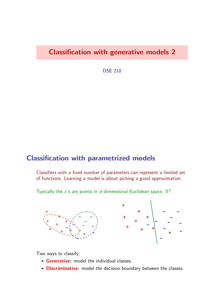
Classification with parametrized models

Classifiers with a fixed number of parameters can represent a limited set

• f functions. Learning a model is about picking a good approximation.

Typically the x’s are points in d-dimensional Euclidean space, Rd. Two ways to classify:

• Generative: model the individual classes.
• Discriminative: model the decision boundary between the classes.

The Bayes-optimal prediction

x Pr(x) P1(x) P2(x) P3(x) π1= 10% π2= 50% π3= 40%

Labels Y = {1, 2, . . . , k}, density Pr(x) = π1P1(x) + · · · + πkPk(x). For any x ∈ X and any label j, Pr(y = j|x) = Pr(y = j)Pr(x|y = j) Pr(x) = πjPj(x) Pk

i=1 πiPi(x)

Bayes-optimal prediction: h∗(x) = arg maxj πjPj(x).

The winery prediction problem

Which winery is it from, 1, 2, or 3? Using one feature (’Alcohol’), error rate is 29%. What if we use two features?

The data set, again

Training set obtained from 130 bottles

• Winery 1: 43 bottles
• Winery 2: 51 bottles
• Winery 3: 36 bottles
• For each bottle, 13 features:

’Alcohol’, ’Malic acid’, ’Ash’, ’Alcalinity of ash’,’Magnesium’, ’Total phenols’, ’Flavanoids’, ’Nonflavanoid phenols’, ’Proanthocyanins’, ’Color intensity’, ’Hue’, ’OD280/OD315 of diluted wines’, ’Proline’ Also, a separate test set of 48 labeled points. This time: ’Alcohol’ and ’Flavanoids’.

Why it helps to add features

Better separation between the classes! Error rate drops from 29% to 8%.

Bivariate distributions

Simplest option: treat each variable as independent. Example: For a large collection of people, measure the two variables H = height W = weight Independence would mean Pr(H = h, W = w) = Pr(H = h) Pr(W = w), which would also imply E(HW ) = E(H)E(W ). Is this an accurate approximation? No: we’d expect height and weight to be positively correlated.

Types of correlation

height weight

H, W positively correlated. This also implies E(HW ) > E(H)E(W ).

Y X

X, Y negatively correlated

Y X

X, Y uncorrelated

Pearson (1903): fathers and sons

58 60 62 64 66 68 70 72 74 76 78 Father’s height (inches) 58 60 62 64 66 68 70 72 74 76 78 Son’s height (inches) Heights of fathers and their full grown sons

How to quantify the degree of correlation?

Correlation pictures

r = 0 r = 1 r = 0.25 r = −0.25 r = 0.5 r = −0.5 r = 0.75 r = −0.75

Covariance and correlation

Suppose X has mean µX and Y has mean µY .

• Covariance

cov(X, Y ) = E[(X − µX)(Y − µY )] = E[XY ] − µXµY Maximized when X = Y , in which case it is var(X). In general, it is at most std(X)std(Y ).

• Correlation

corr(X, Y ) = cov(X, Y ) std(X)std(Y ) This is always in the range [−1, 1].

Covariance and correlation: example 1

cov(X, Y ) = E[(X − µX)(Y − µY )] = E[XY ] − µXµY corr(X, Y ) = cov(X, Y ) std(X)std(Y ) x y Pr(x, y) −1 −1 1/3 −1 1 1/6 1 −1 1/3 1 1 1/6 µX = 0 µY = − 1/3 var(X) = 1 var(Y ) = 8/9 cov(X, Y ) = 0 corr(X, Y ) = 0 In this case, X, Y are independent. Independent variables always have zero covariance and correlation.

Covariance and correlation: example 2

cov(X, Y ) = E[(X − µX)(Y − µY )] = E[XY ] − µXµY corr(X, Y ) = cov(X, Y ) std(X)std(Y ) x y Pr(x, y) −1 −10 1/6 −1 10 1/3 1 −10 1/3 1 10 1/6 µX = 0 µY = 0 var(X) = 1 var(Y ) = 100 cov(X, Y ) = − 10/3 corr(X, Y ) = − 1/3 In this case, X and Y are negatively correlated.

Return to winery example

Better separation between the classes! Error rate drops from 29% to 8%.

The bivariate Gaussian

Model class 1 by a bivariate Gaussian, parametrized by: mean µ = ✓ 13.7 3.0 ◆ and covariance matrix Σ = ✓ 0.20 0.06 0.06 0.12 ◆

The bivariate (2-d) Gaussian

A distribution over (x1, x2) ∈ R2, parametrized by:

• Mean (µ1, µ2) ∈ R2, where µ1 = E(X1) and µ2 = E(X2)
• Covariance matrix Σ =

 Σ11 Σ12 Σ21 Σ22

• where

8 < : Σ11 = var(X1) Σ22 = var(X2) Σ12 = Σ21 = cov(X1, X2) 9 = ; Density is highest at the mean, falls

• ff in ellipsoidal contours.

Density of the bivariate Gaussian

• Mean (µ1, µ2) ∈ R2, where µ1 = E(X1) and µ2 = E(X2)
• Covariance matrix Σ =

 Σ11 Σ12 Σ21 Σ22

• Density p(x1, x2) =

1 2π|Σ|1/2 exp −1 2  x1 − µ1 x2 − µ2 T Σ−1  x1 − µ1 x2 − µ2 !

Bivariate Gaussian: examples

In either case, the mean is (1, 1). Σ =  4 1

• Σ =

 4 1.5 1.5 1

The decision boundary

Go from 1 to 2 features: error rate goes from 29% to 8%. What kind of function is this? And, can we use more features?

DSE 210: Probability and statistics Winter 2018

Worksheet 6 — Generative models 2

• 1. Would you expect the following pairs of random variables to be uncorrelated, positively correlated, or

negatively correlated? (a) The weight of a new car and its price. (b) The weight of a car and the number of seats in it. (c) The age in years of a second-hand car and its current market value.

• 2. Consider a population of married couples in which every wife is exactly 0.9 of her husband’s age. What

is the correlation between husband’s age and wife’s age?

• 3. Each of the following scenarios describes a joint distribution (x, y). In each case, give the parameters
• f the (unique) bivariate Gaussian that satisfies these properties.

(a) x has mean 2 and standard deviation 1, y has mean 2 and standard deviation 0.5, and the correlation between x and y is −0.5. (b) x has mean 1 and standard deviation 1, and y is equal to x.

• 4. Roughly sketch the shapes of the following Gaussians N(µ, Σ). For each, you only need to show a

representative contour line which is qualitatively accurate (has approximately the right orientation, for instance). (a) µ = ✓ 0 ◆ and Σ = ✓ 9 1 ◆ (b) µ = ✓ 0 ◆ and Σ = ✓ 1 −0.75 −0.75 1 ◆

• 5. For each of the two Gaussians in the previous problem, check your answer using Python: draw 100

random samples from that Gaussian and plot it. 6-1

Linear algebra primer

DSE 210

Data as vectors and matrices

1 2 3 4 5 6 1 2 3 4 5 6

Matrix-vector notation

Vector x ∈ Rd: x =        x1 x2 x3 . . . xd        Matrix M ∈ Rr×d: M =      M11 M12 · · · M1d M21 M22 · · · M2d . . . . . . ... . . . Mr1 Mr2 · · · Mrd      Mij = entry at row i, column j

Transpose of vectors and matrices

x =     1 6 3     has transpose xT = M =   1 2 4 3 9 1 6 8 7 2   has transpose MT = .

• (AT)ij = Aji
• (AT)T = A

Adding and subtracting vectors and matrices Dot product of two vectors

Dot product of vectors x, y ∈ Rd: x · y = x1y1 + x2y2 + · · · + xdyd. What is the dot product between these two vectors?

1 2 3 4 1 2 3 4

• 1
• 2
• 3
• 4

x y

Dot products and angles

Dot product of vectors x, y 2 Rd: x · y = x1y1 + x2y2 + · · · + xdyd. Tells us the angle between x and y:

y θ x

cos θ = x · y kxk kyk. x is orthogonal (at right angles) to y if and only if x · y = 0 When x, y are unit vectors (length 1): cos θ = x · y What is x · x?

Linear and quadratic functions

In one dimension:

• Linear: f (x) = 3x + 2
• Quadratic: f (x) = 4x2 2x + 6

In higher dimension, e.g. x = (x1, x2, x3):

• Linear: 3x1 2x2 + x3 + 4
• Quadratic: x2

1 2x1x3 + 6x2 2 + 7x1 + 9

Linear functions and dot products

Linear separator 4x1 + 3x2 = 12:

2 1 4 3 5 1 2 3 4 5

For x = (x1, . . . , xd) ∈ Rd, linear separators are of the form: w1x1 + w2x2 + · · · + wdxd = c. Can write as w · x = c, for w = (w1, . . . , wd).

More general linear functions

A linear function from R4 to R: f (x1, x2, x3, x4) = 3x1 − 2x3 A linear function from R4 to R3: f (x1, x2, x3, x4) = (4x1 − x2, x3, −x1 + 6x4)

Matrix-vector product

Product of matrix M ∈ Rr×d and vector x ∈ Rd:

The identity matrix

The d × d identity matrix Id sends each x ∈ Rd to itself. Id =        1 · · · 1 · · · 1 · · · . . . . . . . . . ... . . . · · · 1       

Matrix-matrix product

Product of matrix A ∈ Rr×k and matrix B ∈ Rk×p:

Matrix products

If A ∈ Rr×k and B ∈ Rk×p, then AB is an r × p matrix with (i, j) entry (AB)ij = (dot product of ith row of A and jth column of B) =

k

X

`=1

Ai`B`j

• IkB = B and A Ik = A
• Can check: (AB)T = BTAT
• For two vectors u, v ∈ Rd, what is uTv?

Some special cases

For vector x ∈ Rd, what are xTx and xxT?

Associative but not commutative

• Multiplying matrices is not commutative: in general,

AB 6= BA ✓1 2 1 ◆ ✓1 1 ◆ = ✓1 1 ◆ ✓1 2 1 ◆ =

• But it is associative: ABCD = (AB)(CD) = (A(BC))D, etc.

Example: if x 2 Rd has length 2, what is xTxxTxxTxxTx?

A special case

Recall: For vector x 2 Rd, we have xTx = kxk2. What about xTMx, for arbitrary d ⇥ d matrix M?

What is xTMx for M = ✓1 2 3 ◆ ?

Quadratic functions

Let M be any d ⇥ d (square) matrix. For x 2 Rd, the mapping x 7! xTMx is a quadratic function from Rd to R: xTMx =

d

X

i,j=1

Mijxixj. What is the quadratic function associated with M = @ 1 2 3 4 5 1 A?

Write the quadratic function f (x1, x2) = x2

1 + 2x1x2 + 3x2 2 using

matrices and vectors.

Special cases of square matrices

• Symmetric: M = MT

  1 2 3 2 4 5 3 5 6   ,   1 2 3 1 2 4 3 4 6  

• Diagonal: M = diag(m1, m2, . . . , md)

diag(1, 4, 7) =   1 4 7  

Determinant of a square matrix

Determinant of A = ✓a b c d ◆ is |A| = ad − bc. Example: A = ✓3 1 1 2 ◆

Inverse of a square matrix

The inverse of a d ⇥ d matrix A is a d ⇥ d matrix B for which AB = BA = Id. Notation: A−1. Example: if A = ✓ 1 2 2 ◆ then A−1 = ✓ 0 1/2 1/2 1/4 ◆ . Check!

Inverse of a square matrix, cont’d

The inverse of a d ⇥ d matrix A is a d ⇥ d matrix B for which AB = BA = Id. Notation: A−1.

• Not all square matrices have an inverse
• Square matrix A is invertible if and only if |A| 6= 0
• What is the inverse of A = diag(a1, . . . , ad)?

DSE 210: Probability and statistics Winter 2018

Worksheet 7 — Linear algebra primer

• 1. Find the unit vector in the same direction as x = (1, 2, 3).
• 2. Find all unit vectors in R2 that are orthogonal to (1, 1).
• 3. How would you describe the set of all points x ∈ Rd with x · x = 25?
• 4. The function f(x) = 2x1 − x2 + 6x3 can be written as w · x for x ∈ R3. What is w?
• 5. For a certain pair of matrices A, B, the product AB has dimension 10 × 20. If A has 30 columns, what

are the dimensions of A and B?

• 6. We have n data points x(1), . . . , x(n) ∈ Rd and we store them in a matrix X, one point per row.

(a) What is the dimension of X? (b) What is the dimension of XXT ? (c) What is the (i, j) entry of XXT , simply?

• 7. Vector x has length 10. What is xT xxT xxT x?
• 8. For x = (1, 3, 5) compute xT x and xxT .
• 9. Vectors x, y ∈ Rd both have length 2. If xT y = 2, what is the angle between x and y?
• 10. The quadratic function f : R3 → R given by

f(x) = 3x2

1 + 2x1x2 − 4x1x3 + 6x2 3

can be written in the form xT Mx for some symmetric matrix M. What is M?

• 11. Which of the following matrices is necessarily symmetric?

(a) AAT for arbitrary matrix A. (b) AT A for arbitrary matrix A. (c) A + AT for arbitrary square matrix A. (d) A − AT for arbitrary square matrix A.

• 12. Let A = diag(1, 2, 3, 4, 5, 6, 7, 8).

(a) What is |A|? (b) What is A−1?

• 13. Vectors u1, . . . , ud ∈ Rd all have unit length and are orthogonal to each other. Let U be the d × d

matrix whose rows are the ui. (a) What is UU T ? (b) What is U −1?

• 14. Matrix A =

✓ 1 2 3 z ◆ is singular. What is z? 7-1

Classification with generative models 3

DSE 210

Recall: the bivariate Gaussian

Bivariate Gaussian, parametrized by: mean µ = ✓ 13.7 3.0 ◆ and covariance matrix Σ = ✓ 0.20 0.06 0.06 0.12 ◆

The multivariate Gaussian

µ N(µ, Σ): Gaussian in Rd

• mean: µ 2 Rd
• covariance: d ⇥ d matrix Σ

Generates points X = (X1, X2, . . . , Xd).

• µ is the vector of coordinate-wise means:

µ1 = EX1, µ2 = EX2, . . . , µd = EXd.

• Σ is a matrix containing all pairwise covariances:

Σij = Σji = cov(Xi, Xj) if i 6= j Σii = var(Xi) Density p(x) = 1 (2π)d/2|Σ|1/2 exp ✓ 1 2(x µ)TΣ−1(x µ) ◆

Special case: independent features

Suppose the Xi are independent, and var(Xi) = σ2

i .

What is the covariance matrix Σ, and what is its inverse Σ−1?

Diagonal Gaussian

Diagonal Gaussian: the Xi are independent, with variances σ2

i . Thus

Σ = diag(σ2

1, . . . , σ2 d) (off-diagonal elements zero)

Each Xi is an independent one-dimensional Gaussian N(µi, σ2

i ):

Pr(x) = Pr(x1)Pr(x2) · · · Pr(xd) = 1 (2π)d/2σ1 · · · σd exp

• d

X

i=1

(xi µi)2 2σ2

i

! Contours of equal density are axis- aligned ellipsoids centered at µ:

σ1

µ

σ2

Even more special case: spherical Gaussian

The Xi are independent and all have the same variance σ2. Σ = σ2Id = diag(σ2, σ2, . . . , σ2) (diagonal elements σ2, rest zero) Each Xi is an independent univariate Gaussian N(µi, σ2): Pr(x) = Pr(x1)Pr(x2) · · · Pr(xd) = 1 (2π)d/2σd exp ✓ kx µk2 2σ2 ◆ Density at a point depends only on its distance from µ:

µ

How to fit a Gaussian to data

Fit a Gaussian to data points x(1), . . . , x(m) ∈ Rd.

• Empirical mean

µ = 1 m ⇣ x(1) + · · · + x(m)⌘

• Empirical covariance matrix has i, j entry:

Σij = 1 m

m

X

k=1

x(k)

i

x(k)

j

! − µiµj

Back to the winery data

Go from 1 to 2 features: test error goes from 29% to 8%. With all 13 features: test error rate goes to zero.

The multivariate Gaussian

µ

N(µ, Σ): Gaussian in Rd

• mean: µ ∈ Rd
• covariance: d × d matrix Σ

Density p(x) = 1 (2π)d/2|Σ|1/2 exp ✓ −1 2(x − µ)TΣ−1(x − µ) ◆ If we write S = Σ−1 then S is a d × d matrix and (x − µ)TΣ−1(x − µ) = X

i,j

Sij(xi − µi)(xj − µj), a quadratic function of x.

Binary classification with Gaussian generative model

• Estimate class probabilities π1, π2
• Fit a Gaussian to each class: P1 = N(µ1, Σ1), P2 = N(µ2, Σ2)

Given a new point x, predict class 1 if π1P1(x) > π2P2(x) ⇔ xTMx + 2w Tx ≥ θ, where: M = 1 2(Σ−1

2

− Σ−1

1 )

w = Σ−1

1 µ1 − Σ−1 2 µ2

and θ is a threshold depending on the various parameters. Linear or quadratic decision boundary.

Common covariance: Σ1 = Σ2 = Σ

Linear decision boundary: choose class 1 if x · Σ−1(µ1 − µ2) | {z }

w

≥ θ. Example 1: Spherical Gaussians with Σ = Id and π1 = π2. µ1

µ2

w

bisector of line joining means

Example 2: Again spherical, but now π1 > π2. µ1

µ2

w

Example 3: Non-spherical.

µ1

µ2

µ1 − µ2

w = Σ−1(µ1 − µ2) Classification rule: w · x θ

• Choose w as above
• Common practice: fit θ to minimize training or validation error

Different covariances: Σ1 6= Σ2

Quadratic boundary: choose class 1 if xTMx + 2w Tx θ, where: M = 1 2(Σ−1

2

Σ−1

1 )

w = Σ−1

1 µ1 Σ−1 2 µ2

Example 1: Σ1 = σ2

1Id and Σ2 = σ2 2Id with σ1 > σ2 µ1 µ2

Example 2: Same thing in 1-d. X = R.

class 1 class 2

Example 3: A parabolic boundary. µ1

µ2

Multiclass discriminant analysis

k classes: weights πj, class-conditional densities Pj = N(µj, Σj). Each class has an associated quadratic function fj(x) = log (πj Pj(x)) To classify point x, pick arg maxj fj(x). If Σ1 = · · · = Σk, the boundaries are linear.

Beyond Gaussians

The generative methodology:

• Fit a distribution to each class separately
• Use Bayes’ rule to classify new data

What distribution to use? Are Gaussians enough?

Exponential families of distributions

It was the best of times, it was the

worst of times, it was the age of wisdom, it was the age of foolishness, it was the epoch of belief, it was the epoch of incredulity, it was the season of Light, it was the season of Darkness, it was the spring of hope, it was the winter of despair, we had everything before us, we had nothing before us, we were all going direct to Heaven, we were all going direct the

• ther way – in short, the period was

so far like the present period, that some of its noisiest authorities insisted on its being received, for good or for evil, in the superlative degree of comparison only.

despair evil happiness foolishness 1 1 2

GAMMA BETA POISSON CATEGORICAL

Multivariate distributions

We’ve described a variety of distributions for one-dimensional data. What about higher dimensions?

1 Naive Bayes: Treat coordinates as independent.

For x = (x1, . . . , xd), fit separate models Pri to each xi, and assume Pr(x1, . . . , xd) = Pr1(x1)Pr2(x2) · · · Prd(xd). This assumption is typically inaccurate.

2 Multivariate Gaussian.

Model correlations between features: we’ve seen this in detail.

3 Graphical models.

Arbitrary dependencies between coordinates.

Handling text data

Bag-of-words: vectorial representation of text documents.

It was the best of times, it was the

worst of times, it was the age of wisdom, it was the age of foolishness, it was the epoch of belief, it was the epoch of incredulity, it was the season of Light, it was the season of Darkness, it was the spring of hope, it was the winter of despair, we had everything before us, we had nothing before us, we were all going direct to Heaven, we were all going direct the

• ther way – in short, the period was

so far like the present period, that some of its noisiest authorities insisted on its being received, for good or for evil, in the superlative degree of comparison only.

despair evil happiness foolishness 1 1 2

• Fix V = some vocabulary.
• Treat each document as a vector of length |V |:

x = (x1, x2, . . . , x|V |), where xi = # of times the ith word appears in the document. A standard distribution over such document-vectors x: the multinomial.

Multinomial naive Bayes

Multinomial distribution over a vocabulary V : p = (p1, . . . , p|V |), such that pi ≥ 0 and X

i

pi = 1 Document x = (x1, . . . , x|V |) has probability ∝ px1

1 px2 2 · · · p x|V | |V | .

For naive Bayes: one multinomial distribution per class.

• Class probabilities π1, . . . , πk
• Multinomials p(1) = (p11, . . . , p1|V |), . . . , p(k) = (pk1, . . . , pk|V |)

Classify document x as arg max

j

πj

|V |

Y

i=1

pxi

ji .

(As always, take log to avoid underflow: linear classifier.)

Improving performance of multinomial naive Bayes

A variety of heuristics that are standard in text retrieval, such as:

1 Compensating for burstiness.

Problem: Once a word has appeared in a document, it has a much higher chance of appearing again. Solution: Instead of the number of occurrences f of a word, use log(1 + f ).

2 Downweighting common words.

Problem: Common words can have a unduly large influence on classification. Solution: Weight each word w by inverse document frequency: log # docs #(docs containing w)

DSE 210: Probability and statistics Winter 2018

Worksheet 8 — Generative models 3

• 1. Consider the linear classifier w · x ≥ θ, where

w = ✓ −3 4 ◆ and θ = 12. Sketch the decision boundary in R2. Make sure to label precisely where the boundary intersects the coordinate axes, and also indicate which side of the boundary is the positive side.

• 2. How many parameters are needed to specify a diagonal Gaussian in Rd?
• 3. Text classification using multinomial Naive Bayes.

(a) For this problem, you’ll be using the 20 Newsgroups data set. There are several versions of it on the web. You should download “20news-bydate.tar.gz” from http://qwone.com/~jason/20Newsgroups/ Unpack it and look through the directories at some of the files. Overall, there are roughly 19,000 documents, each from one of 20 newsgroups. The label of a document is the identity of its

• newsgroup. The documents are divided into a training set and a test set.

(b) The same website has a processed version of the data, “20news-bydate-matlab.tgz”, that is par- ticularly convenient to use. Download this and also the file “vocabulary.txt”. Look at the first training document in the processed set and the corresponding original text document to under- stand the relation between the two. (c) The words in the documents constitute an overall vocabulary V of size 61188. Build a multinomial Naive Bayes model using the training data. For each of the 20 classes j = 1, 2, . . . , 20, you must have the following:

• πj, the fraction of documents that belong to that class; and
• Pj, a probability distribution over V that models the documents of that class.

In order to fit Pj, imagine that all the documents of class j are strung together. For each word w ∈ V , let Pjw be the fraction of this concatenated document occupied by w. Well, almost: you will need to do smoothing (just add one to the count of how often w occurs). (d) Write a routine that uses this naive Bayes model to classify a new document. To avoid underflow, work with logs rather than multiplying together probabilities. (e) Evaluate the performance of your model on the test data. What error rate do you achieve? (f) If you have the time and inclination: see if you can get a better-performing model.

• Split the training data into a smaller training set and a validation set. The split could be

80-20, for instance. You’ll use this training set to estimate parameters and the validation set to decide between different options. 8-1

DSE 210 Worksheet 8 — Generative models 3 Winter 2018

• Think of 2-3 ways in which you might improve your earlier model. Examples include: (i)

replacing the frequency f of a word in a document by log(1 + f), (ii) removing stopwords; (iii) reducing the size of the vocabulary; etc. Estimate a revised model for each of these, and use the validation set to choose between them.

• Evaluate your final model on the test data. What error rate do you achieve?
• 4. Handwritten digit recognition using a Gaussian generative model. In class, we mentioned the MNIST

data set of handwritten digits. You can obtain it from: http://yann.lecun.com/exdb/mnist/index.html In this problem, you will build a classifier for this data, by modeling each class as a multivariate (784-dimensional) Gaussian. (a) Upon downloading the data, you should have two training files (one with images, one with labels) and two test files. Unzip them. In order to load the data into Python you will find the following code helpful: http://cseweb.ucsd.edu/~dasgupta/dse210/loader.py For instance, to load in the training data, you can use: x,y = loadmnist(’train-images-idx3-ubyte’, ’train-labels-idx1-ubyte’) This will set x to a 60000 × 784 array where each row corresponds to an image, and y to a length-60000 array where each entry is a label (0-9). There is also a routine to display images: use displaychar(x[0]) to show the first data point, for instance. (b) Split the training set into two pieces – a training set of size 50000, and a separate validation set

• f size 10000. Also load in the test data.

(c) Now fit a Gaussian generative model to the training data of 50000 points:

• Determine the class probabilities: what fraction π0 of the training points are digit 0, for

instance? Call these values π0, . . . , π9.

• Fit a Gaussian to each digit, by finding the mean and the covariance of the corresponding

data points. Let the Gaussian for the jth digit be Pj = N(µj, Σj). Using these two pieces of information, you can classify new images x using Bayes’ rule: simply pick the digit j for which πjPj(x) is largest. (d) One last step is needed: it is important to smooth the covariance matrices, and the usual way to do this is to add in cI, where c is some constant and I is the identity matrix. What value of c is right? Use the validation set to help you choose. That is, choose the value of c for which the resulting classifier makes the fewest mistakes on the validation set. What value of c did you get? (e) Turn in an iPython notebook that includes:

• All your code.
• Error rate on the MNIST test set.
• Out of the misclassified test digits, pick five at random and display them. For each instance,

list the posterior probabilities Pr(y|x) of each of the ten classes. 8-2