
SLIDE 1
Fundamentals of Power Electronics
1
Chapter 11: Current Programmed Control
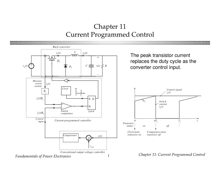
Chapter 11 Current Programmed Control
+ – Buck converter Current-programmed controller R vg(t) is(t) + v(t) – iL(t) Q1 L C D1
+ –
Analog comparator Latch
Ts
S R Q Clock
is(t) Rf
Measure switch current
is(t)Rf
Control input
ic(t)Rf –+ vref v(t)
Compensator
Conventional output voltage controller
Switch current is(t) Control signal ic(t) m1
t
dTs Ts
- n
- ff
Transistor status: Clock turns transistor on Comparator turns transistor off