CCD Image Processing: CCD Image Processing: [ ] [ ] r x y , - - PDF document

1

CCD Image Processing: CCD Image Processing: Issues & Solutions Issues & Solutions

[ ] [ ]

, , r x y d x y −

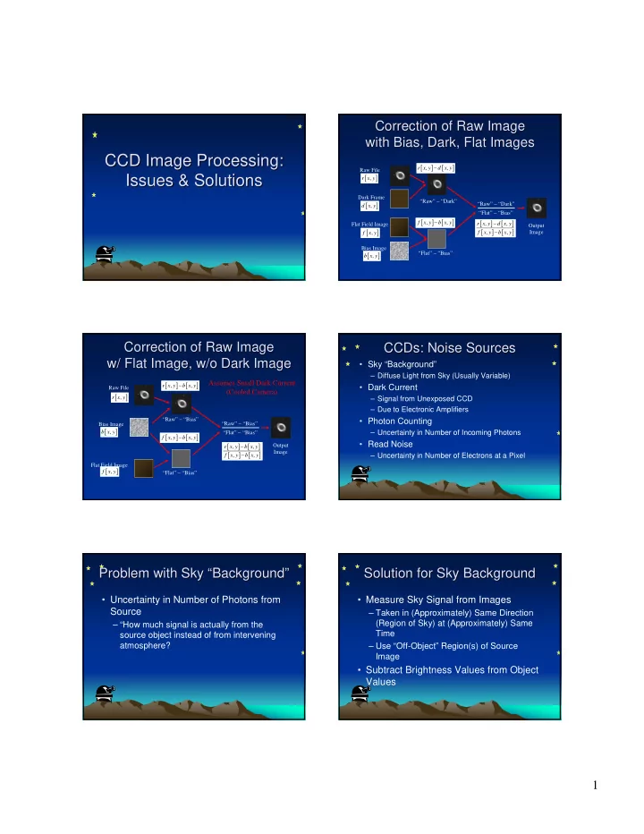
Correction of Raw Image Correction of Raw Image with Bias, Dark, Flat Images with Bias, Dark, Flat Images

Flat Field Image Bias Image Output Image Dark Frame Raw File

[ ]

, r x y

[ ]

, d x y

[ ]

, f x y

[ ]

, b x y

[ ] [ ]

, , f x y b x y − “Flat” − “Bias” “Raw” − “Dark”

[ ] [ ] [ ] [ ]

, , , , r x y d x y f x y b x y − − “Raw” − “Dark” “Flat” − “Bias”

[ ] [ ]

, , r x y b x y −

Correction of Raw Image Correction of Raw Image w/ Flat Image, w/o Dark Image w/ Flat Image, w/o Dark Image

Flat Field Image Bias Image Output Image Raw File

[ ]

, r x y

[ ]

, f x y

[ ]

, b x y

[ ] [ ]

, , f x y b x y − “Flat” − “Bias”

[ ] [ ] [ ] [ ]

, , , , r x y b x y f x y b x y − − “Raw” − “Bias” “Flat” − “Bias” “Raw” − “Bias”

Assumes Small Dark Current (Cooled Camera)

CCDs CCDs: Noise Sources : Noise Sources

• Sky “Background”

– Diffuse Light from Sky (Usually Variable)

• Dark Current

– Signal from Unexposed CCD – Due to Electronic Amplifiers

• Photon Counting

– Uncertainty in Number of Incoming Photons

• Read Noise

– Uncertainty in Number of Electrons at a Pixel

Problem with Sky Problem with Sky “ “Background Background” ”

• Uncertainty in Number of Photons from

Source

– “How much signal is actually from the source object instead of from intervening atmosphere?

Solution for Sky Background Solution for Sky Background

• Measure Sky Signal from Images

– Taken in (Approximately) Same Direction (Region of Sky) at (Approximately) Same Time – Use “Off-Object” Region(s) of Source Image

• Subtract Brightness Values from Object

Values

2

Problem: Dark Current Problem: Dark Current

• Signal in Every Pixel Even if NOT

Exposed to Light

– Strength Proportional to Exposure Time

• Signal Varies Over Pixels

– Non-Deterministic Signal = “NOISE”

Solution: Dark Current Solution: Dark Current

• Subtract Image(s) Obtained Without

Exposing CCD

– Leave Shutter Closed to Make a “Dark Frame” – Same Exposure Time for Image and Dark Frame

• Measure of “Similar” Noise as in Exposed Image
• Actually Average Measurements from Multiple

Images

– Decreases “Uncertainty” in Dark Current

Digression on Digression on “ “Noise Noise” ”

• What is “Noise”?
• Noise is a “Nondeterministic” Signal

– “Random” Signal – Exact Form is not Predictable – “Statistical” Properties ARE (usually) Predictable

Statistical Properties of Noise Statistical Properties of Noise

• 1. Average Value = “Mean” ≡ µ
• 2. Variation from Average = “Deviation” ≡ σ
• Distribution of Likelihood of Noise

– “Probability Distribution”

• More General Description of Noise than µ, σ

– Often Measured from Noise Itself

• “Histogram”

Histogram of Histogram of “ “Uniform Distribution Uniform Distribution” ”

• Values are “Real Numbers” (e.g., 0.0105)
• Noise Values Between 0 and 1 “Equally” Likely
• Available in Computer Languages

Variation Mean µ

Mean µ = 0.5

Mean µ Variation

Noise Sample Histogram

Histogram of Histogram of “ “Gaussian Gaussian” ” Distribution Distribution

• Values are “Real Numbers”
• NOT “Equally” Likely
• Describes Many Physical Noise Phenomena

Mean µ = 0 Values “Close to” µ “More Likely”

Variation Mean µ Mean µ Variation

3

Histogram of Histogram of “ “Poisson Poisson” ” Distribution Distribution

• Values are “Integers” (e.g., 4, 76, …)
• Describes Distribution of “Infrequent” Events,

e.g., Photon Arrivals

Mean µ = 4 Values “Close to” µ “More Likely” “Variation” is NOT Symmetric

Variation Mean µ Mean µ Variation

Histogram of Histogram of “ “Poisson Poisson” ” Distribution Distribution

Mean µ = 25

Variation Mean µ Mean µ Variation

How to Describe How to Describe “ “Variation Variation” ”: 1 : 1

• Measure of the “Spread” (“Deviation”) of

the Measured Values (say “x”) from the “Actual” Value, which we can call “µ”

• The “Error” ε of One Measurement is:

(which can be positive or negative)

( )

x ε µ = −

Description of Description of “ “Variation Variation” ”: 2 : 2

• Sum of Errors over all Measurements:

Can be Positive or Negative

• Sum of Errors Can Be Small, Even If

Errors are Large (Errors can “Cancel”)

( )

n n n n

x ε µ = −

∑ ∑

Description of Description of “ “Variation Variation” ”: 3 : 3

• Use “Square” of Error Rather Than Error

Itself: Must be Positive

( )

2 2

x ε µ = − ≥

Description of Description of “ “Variation Variation” ”: 4 : 4

• Sum of Squared Errors over all

Measurements:

• Average of Squared Errors

( ) ( )

2 2 n n n n

x ε µ = − ≥

∑ ∑

( ) ( )

2 2

1

n n n n

x N N µ ε − = ≥

∑ ∑

4

Description of Description of “ “Variation Variation” ”: 5 : 5

• Standard Deviation σ = Square Root of

Average of Squared Errors

( )

2 n n

x N µ σ − ≡ ≥

∑

Effect of Averaging on Deviation Effect of Averaging on Deviation σ σ

• Example: Average of 2 Readings from

Uniform Distribution

Effect of Averaging of 2 Samples: Effect of Averaging of 2 Samples: Compare the Histograms Compare the Histograms

• Averaging Does Not Change µ
• “Shape” of Histogram is Changed!

– More Concentrated Near µ – Averaging REDUCES Variation σ

σ ≅ 0.289

Mean µ Mean µ

Averaging Reduces Averaging Reduces σ σ

σ ≅ 0.289 σ ≅ 0.205

σ is Reduced by Factor:

41 . 1 205 . 289 . ≅

Averages of 4 and 9 Samples Averages of 4 and 9 Samples

σ ≅ 0.144 σ ≅ 0.096

Reduction Factors

01 . 2 144 . 289 . ≅ 01 . 3 096 . 289 . ≅

Averaging of Random Noise Averaging of Random Noise REDUCES the Deviation REDUCES the Deviation σ σ

3.01 2.01 1.41 Reduction in Deviation σ N = 9 N = 4 N = 2 Samples Averaged

Observation:

One Sample Average of N Samples

N σ σ =

5

Why Does Why Does “ “Deviation Deviation” ” Decrease Decrease if Images are Averaged? if Images are Averaged?

• “Bright” Noise Pixel in One Image may be

“Dark” in Second Image

• Only Occasionally Will Same Pixel be

“Brighter” (or “Darker”) than the Average in Both Images

• “Average Value” is Closer to Mean Value

than Original Values

Averaging Over Averaging Over “ “Time Time” ” vs. vs. Averaging Over Averaging Over “ “Space Space” ”

• Examples of Averaging Different Noise

Samples Collected at Different Times

• Could Also Average Different Noise Samples

Over “Space” (i.e., Coordinate x)

– “Spatial Averaging”

Comparison of Histograms After Comparison of Histograms After Spatial Averaging Spatial Averaging

Uniform Distribution µ = 0.5 σ ≅ 0.289 Spatial Average

• f 4 Samples

µ = 0.5 σ ≅ 0.144 Spatial Average

• f 9 Samples

µ = 0.5 σ ≅ 0.096

Effect of Averaging on Dark Effect of Averaging on Dark Current Current

• Dark Current is NOT a “Deterministic”

Number

– Each Measurement of Dark Current “Should Be” Different – Values Are Selected from Some Distribution of Likelihood (Probability)

Example of Dark Current Example of Dark Current

• One-Dimensional Examples (1-D

Functions)

– Noise Measured as Function of One Spatial Coordinate

Example of Dark Current Example of Dark Current Readings Readings

Variation

Reading of Dark Current vs. Position in Simulated Dark Image #1 Reading of Dark Current vs. Position in Simulated Dark Image #2

6

Averages of Independent Dark Averages of Independent Dark Current Readings Current Readings

Variation

Average of 2 Readings of Dark Current vs. Position Average of 9 Readings of Dark Current vs. Position

“Variation” in Average of 9 Images ≅ 1/√9 = 1/3 of “Variation” in 1 Image

Infrequent Photon Arrivals Infrequent Photon Arrivals

• Different Mechanism

– Number of Photons is an “Integer”!

• Different Distribution of Values

Problem: Photon Counting Problem: Photon Counting Statistics Statistics

• Photons from Source Arrive

“Infrequently”

– Few Photons

• Measurement of Number of Source

Photons (Also) is NOT Deterministic

– Random Numbers – Distribution of Random Numbers of “Rarely Occurring” Events is Governed by Poisson Statistics

Simplest Distribution of Integers Simplest Distribution of Integers

• Only Two Possible Outcomes:

– YES – NO

• Only One Parameter in Distribution

– “Likelihood” of Outcome YES – Call it “p” – Just like Counting Coin Flips – Examples with 1024 Flips of a Coin

Example with Example with p = p = 0.5 0.5

N = 1024 Nheads = 511 p = 511/1024 < 0.5 String of Outcomes Histogram N = 1024 Nheads = 522 µ = 522/1024 > 0.5 String of Outcomes Histogram

Second Example with Second Example with p p = 0.5 = 0.5

“H” “T”

7

What if Coin is What if Coin is “ “Unfair Unfair” ”? ? p p ≠ ≠ 0.5 0.5

String of Outcomes Histogram “H” “T”

What Happens to Deviation What Happens to Deviation σ σ? ?

• For One Flip of 1024 Coins:

– p = 0.5 ⇒ σ ≅ 0.5 – p = 0 ⇒ ? – p = 1 ⇒ ?

Deviation is Largest if Deviation is Largest if p p = 0.5! = 0.5!

• The Possible Variation is Largest if p is in

the middle!

Add More Add More “ “Tosses Tosses” ”

• 2 Coin Tosses ⇒ More Possibilities for

Photon Arrivals

N = 1024 µ = 1.028 String of Outcomes Histogram

Sum of Two Sets with Sum of Two Sets with p p = 0.5 = 0.5

3 Outcomes:

• 2 H
• 1H, 1T (most likely)
• 2T

N = 1024 String of Outcomes Histogram

Sum of Two Sets with Sum of Two Sets with p p = 0.25 = 0.25

3 Outcomes:

• 2 H (least likely)
• 1H, 1T
• 2T (most likely)

8

Add More Flips with Add More Flips with “ “Unlikely Unlikely” ” Heads Heads

Most “Pixels” Measure 25 Heads (100 × 0.25)

Add More Flips with Add More Flips with “ “Unlikely Unlikely” ” Heads (1600 with Heads (1600 with p = p = 0.25) 0.25)

Most “Pixels” Measure 400 Heads (1600 × 0.25)

Examples of Poisson Examples of Poisson “ “Noise Noise” ” Measured at 64 Pixels Measured at 64 Pixels

Average Value µ = 25 Average Values µ = 400 AND µ = 25

• 1. Exposed CCD to Uniform Illumination
• 2. Pixels Record Different Numbers of Photons

“ “Variation Variation” ” of Measurement

• f Measurement

Varies with Number of Photons Varies with Number of Photons

• For Poisson-Distributed Random Number

with Mean Value µ = N:

• “Standard Deviation” of Measurement is:

σ = √N

Average Value µ = 400 Variation σ = √400 = 20

Histograms of Two Poisson Histograms of Two Poisson Distributions Distributions

µ = 25 µ=400 Variation Variation Average Value µ = 25 Variation σ = √25 = 5

(Note: Change of Horizontal Scale!)

“ “Quality Quality” ” of Measurement of

• f Measurement of

Number of Photons Number of Photons

• “Signal-to-Noise Ratio”

– Ratio of “Signal” to “Noise” (Man, Like What Else?)

SNR µ σ ≡

9

Signal Signal-

• to

to-

• Noise Ratio for

Noise Ratio for Poisson Distribution Poisson Distribution

• “Signal-to-Noise Ratio” of Poisson Distribution
• More Photons ⇒ Higher-Quality Measurement

N SNR N N µ σ ≡ = =

Solution: Photon Counting Solution: Photon Counting Statistics Statistics

• Collect as MANY Photons as POSSIBLE!!
• Largest Aperture (Telescope Collecting Area)
• Longest Exposure Time
• Maximizes Source Illumination on Detector

– Increases Number of Photons

• Issue is More Important for X Rays than for

Longer Wavelengths

– Fewer X-Ray Photons

Problem: Read Noise Problem: Read Noise

• Uncertainty in Number of Electrons

Counted

– Due to Statistical Errors, Just Like Photon Counts

• Detector Electronics

Solution: Read Noise Solution: Read Noise

• Collect Sufficient Number of Photons so

that Read Noise is Less Important Than Photon Counting Noise

• Some Electronic Sensors (CCD-“like”

Devices) Can Be Read Out “Nondestructively”

– “Charge Injection Devices” (CIDs) – Used in Infrared

• multiple reads of CID pixels reduces

uncertainty

CCDs CCDs: artifacts and defects : artifacts and defects

1. Bad Pixels

– dead, hot, flickering…

2. Pixel-to-Pixel Differences in Quantum Efficiency (QE)

– 0 ≤ QE < 1 – Each CCD pixel has its “own” unique QE – Differences in QE Across Pixels ⇒ Map of CCD “Sensitivity”

• Measured by “Flat Field”

# of electrons created Quantum Efficiency # of incident photons =

CCDs CCDs: artifacts and defects : artifacts and defects

3. Saturation

– each pixel can hold a limited quantity of electrons (limited well depth of a pixel)

4. Loss of Charge during pixel charge transfer & readout

– Pixel’s Value at Readout May Not Be What Was Measured When Light Was Collected

10

Bad Pixels Bad Pixels

• Issue: Some Fraction of Pixels in a CCD are:

– “Dead” (measure no charge) – “Hot” (always measure more charge than collected)

• Solutions:

– Replace Value of Bad Pixel with Average of Pixel’s Neighbors – Dither the Telescope over a Series of Images

• Move Telescope Slightly Between Images to Ensure that

Source Fall on Good Pixels in Some of the Images

• Different Images Must be “Registered” (Aligned) and

Appropriately Combined

Pixel Pixel-

• to

to-

• Pixel Differences in QE

Pixel Differences in QE

• Issue: each pixel has its own response to light
• Solution: obtain and use a flat field image to

correct for pixel-to-pixel nonuniformities

– construct flat field by exposing CCD to a uniform source of illumination

• image the sky or a white screen pasted on the dome

– divide source images by the flat field image

• for every pixel x,y, new source intensity is now

S’(x,y) = S(x,y)/F(x,y) where F(x,y) is the flat field pixel value; “bright” pixels are suppressed, “dim” pixels are emphasized

Issue: Saturation Issue: Saturation

• Issue: each pixel can only hold so many electrons

(limited well depth of the pixel), so image of bright source often saturates detector

– at saturation, pixel stops detecting new photons (like overexposure) – saturated pixels can “bleed” over to neighbors, causing streaks in image

• Solution: put less light on detector in each image

– take shorter exposures and add them together

• telescope pointing will drift; need to re-register images
• read noise can become a problem

– use neutral density filter

• a filter that blocks some light at all wavelengths uniformly
• fainter sources lost

Solution to Saturation Solution to Saturation

• Reduce Light on Detector in Each Image

– Take a Series of Shorter Exposures and Add Them Together

• Telescope Usually “Drifts”

– Images Must be “Re-Registered”

• Read Noise Worsens

– Use Neutral Density Filter

• Blocks Same Percentage of Light at All Wavelengths
• Fainter Sources Lost

Issue: Loss of Electron Charge Issue: Loss of Electron Charge

• No CCD Transfers Charge Between

Pixels with 100% Efficiency

– Introduces Uncertainty in Converting to Light Intensity (of “Optical” Visible Light) or to Photon Energy (for X Rays)

• Build Better CCDs!!!
• Increase Transfer Efficiency
• Modern CCDs have charge transfer

efficiencies ≥ 99.9999%

– some do not: those sensitive to “soft” X Rays

• longer wavelengths than short-wavelength “hard” X

Rays

Solution to Loss of Electron Solution to Loss of Electron Charge Charge

# of electrons transferred to next pixel Transfer Efficiency # of electrons in pixel =

11

Digital Processing of Digital Processing of Astronomical Images Astronomical Images

• Computer Processing of Digital Images
• Arithmetic Calculations:

– Addition – Subtraction – Multiplication – Division

Digital Processing Digital Processing

• Images are Specified as “Functions”, e.g.,

r [x,y]

means the “brightness” r at position [x,y]

• “Brightness” is measured in “Number of Photons”
• [x,y] Coordinates Measured in:

– Pixels – Arc Measurements (Degrees-ArcMinutes- ArcSeconds)

• “Summation” = “Mathematical Integration”
• To “Average Noise”

Sum of Two Images Sum of Two Images

[ ] [ ] [ ]

1 2

, , , r x y r x y g x y + =

• To Detect Changes in the Image, e.g., Due

to Motion

Difference of Two Images Difference of Two Images

[ ] [ ] [ ]

1 2

, , , r x y r x y g x y − =

• m[x,y] is a “Mask” Function

Multiplication of Two Images Multiplication of Two Images

[ ] [ ] [ ]

, , , r x y m x y g x y × =

• Divide by “Flat Field” f[x,y]

Division of Two Images Division of Two Images

[ ] [ ] [ ]

, , , r x y g x y f x y =

12

Data Pipelining Data Pipelining

• Issue: now that I’ve collected all of these

images, what do I do?

• Solution: build an automated data processing

pipeline

– Space observatories (e.g., HST) routinely process raw image data and deliver only the processed images to the

• bserver

– ground-based observatories are slowly coming around to this operational model – RIT’s CIS is in the “data pipeline” business

• NASA’s SOFIA
• South Pole facilities