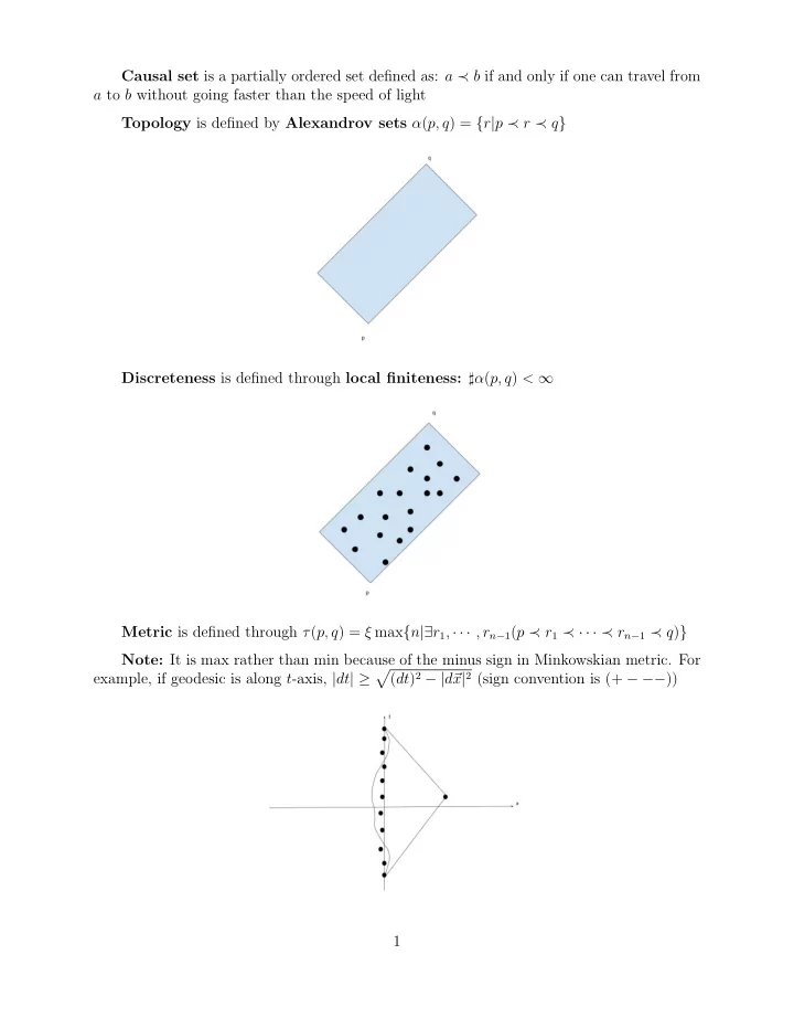
SLIDE 1 Causal set is a partially ordered set defined as: a ≺ b if and only if one can travel from a to b without going faster than the speed of light Topology is defined by Alexandrov sets α(p, q) = {r|p ≺ r ≺ q} Discreteness is defined through local finiteness: ♯α(p, q) < ∞ Metric is defined through τ(p, q) = ξ max{n|∃r1, · · · , rn−1(p ≺ r1 ≺ · · · ≺ rn−1 ≺ q)} Note: It is max rather than min because of the minus sign in Minkowskian metric. For example, if geodesic is along t-axis, |dt| ≥
x|2 (sign convention is (+ − −−)) 1
SLIDE 2
Key idea a) Assume smooth manifold and the presence of coordinates b) Re-express coordinate-dependent expressions in a way that coordinates aren’t explic- itly mentioned c) Copy the result for the non-manifold situation (ex: tree-like causal structure, etc) Key difference between causal sets and other discrete theories: In manifold situation, the causal set assumption is Poisson scattering = ⇒ lack of structure, emphasis on statistical properties Key difference between my work and other types of causal set theory: I am trying to re-interpret causal structure, the definition of fields, etc, while still sticking to statistical approach 2
SLIDE 3 Conventional version of causal set Lagrangian (Sorkin at el)
Use −φ∆φ instead of +∂µφ∂µφ 2D case: (∆φ)(p) =
(φ(p) + φ(r) − 2φ(s)) (1) d dimension ∆φ =
(c0(d)φ(p) + c1(d)φ(r1) + · · · + cn(d)(d)φ(rn(d))) (2) NOTE Cancelation only occurs sufficiently far away from the boundary What I don’t like about it: Existence of the boundary = ⇒ Preferred frame = ⇒ invalidation of stated claim of causal set theory 3
SLIDE 4
Steven Johnston’s propagator
Summing over all possible paths 1) Propagators are defined direction, WITHOUT the use of Lagrangians 2) Propagators don’t face the problem of non-locality because of the TWO endpoints Problem: Coupling different propagators to each other during φ4-coupling Easy solution: Impose a condition by hand which edges are allowed to be φ4-coupled and which aren’t 4
SLIDE 5
DILLEMA: Locality = ⇒ Finately many neighbors = ⇒ Nearest neighbor = ⇒ Preferred frame MY ANSWER: The price for nearest edge neighbor is violation of Newtons first law INSTEAD OF preferred frame a) the nearest edge-neighbor relates to the fact that geodesic wiggles b) wiggling of geodesic is interpretted as gravity THEREFORE c) nearest edge-neighbor phenomenon is ”explained away” through gravity 5
SLIDE 6 Conventional thinking a(p, q) =
Aµ(γ(τ))˙ γµ(τ)dτ (3) where γ is a geodesic connecting p and q φ(x) is given My thinking a) Replace Aµ(x) and φ(x) with Aµ(x, p) and φ(x, p) b) Assume Aµ(x, p1) ≈ Aµ(x, p2) and φ(x, p1) ≈ φ(x, p2) if the relative velocity of refer- ence frames corresponding to p1 and p2 is not too close to c c) Assume that in the reference frames, with resect to which p/|p| isn’t too close to c, φ(x, p) and Aµ(x, p) are both locally linear d) Define a(p, q) =
Aµ(γ(τ), ˙ γ(τ)) ˙ xµ(τ)dτdτ (4) φ(p, q) = 1 τ(p, q)
φ(γ(τ), ˙ γ(τ)) ˙ xµ(τ)dτ (5) NOTE: Since path integral is dominated by NON-DIFFERENTIABLE paths, the ssumptions b and c are dropped once we are under the path integral; those assumptions ONLY apply to “well behaved” functions we are thinking of in order to “motivate” our definition of the action. NOTE: a(p, q) = −a(q, p), BUT φ(p, q) = +φ(q, p) 6
SLIDE 7 Setup
L = ηscal
(K1(φ; p, q, r) − Cscal(d)K2(φ; p, q)) (6) K1 =
ddr(top − bottom)2 =
ddr(φ(r, q) − φ(p, r))2 (7) K1 =
ddr
e0 2
e0 2 2 =
ddr ∂φ ∂x0
= ∂φ ∂x0
α(p,q)
ddr (8) K2 =
ddr(left − right)2 =
ddr φ(p, r) + φ(r, q) 2 − φ(p, q) 2 (9) K2 =
ddr
r 2
2 =
ddr ∂φ ∂r0
2 + ∂φ ∂r0
2 2 = = 1 4 ∂φ ∂r0
α(p,q)
ddr(r0)2 + ∂φ ∂r1
α(p,q)
ddr(r1)2 + 2 ∂φ ∂r0 ∂φ ∂r1
ddrr0r1
Odd Function = ⇒
ddr r0r1 = 0 (11) K2 = 1 4 ∂φ ∂r0
α(p,q)
ddr(r0)2 + ∂φ ∂r1
α(p,q)
ddr(r1)2
7
SLIDE 8 Finding Cscal(d)
∂φ ∂x0
− Cscal(d) 4
∂φ ∂x0
+ (r1)2 ∂φ ∂x1
= =
4 t2 ∂φ ∂x0
− Cscal(d) 4 (r1)2 ∂φ ∂x1
(13) 1−Cscal(d) 4 t2 = Cscal(d) 4 (r1)2 = ⇒ 1 = Cscal(d) 4 (t2+(r1)2 = ⇒ Cscal(d) = 4 t2 + (r1)2 ξ = 1 − t = ⇒ (1 − t)k = 1
0 ξkξd−1dξ
1
0 ξd−1dξ
= 1
0 ξd+k−1dξ
1
0 ξd−1dξ
=
1 d+k 1 d
= d d + k (14) t = 1 − 1 − t = 1 − d d + 1 = 1 d + 1 (15) t2 = (1 − (1 − t))2 = 1 − 21 − t + (1 − t)2 = 1 − 2d d + 1 + d d + 2 = = (d + 1)(d + 2) − 2d(d + 2) + d(d + 1) (d + 1)(d + 2) = d2 + 3d + 2 − 2d2 − 4d + d2 + d (d + 1)(d + 2) = = (1 − 2 + 1)d2 + (3 − 4 + 1)d + 2 (d + 1)(d + 2) = 2 (d + 1)(d + 2) (16) r2 = 1
0 r2rd−2(1 − r)dr
1
0 rd−2(1 − r)dr
= 1
0 (rd − rd+1)dr
1
0 (rd−2 − rd−1)dr
=
1 d+1 − 1 d+2 1 d−1 − 1 d
= =
d+2−d−1 (d+1)(d+2) d−d+1 (d−1)d
=
1 (d+1)(d+2) 1 (d−1)d
= (d − 1)d (d + 1)(d + 2) (17) r2 =
d−1
(xk)2 = (d − 1)(x1)2 = ⇒ (x1)2 = 1 d − 1r2 = d (d + 1)(d + 2) (18) Cscal(d) = 4 t2 + (x1)2 = 4
2 (d+1)(d+2) + d (d+1)(d+2)
= 4
d+2 (d+1)(d+2)
= 4
1 d+1
= 4(d + 1) (19) 8
SLIDE 9 Avoiding C(d)
K1(f; p1, q1) − C(d)K2(f; p1, q1) = K1(f; p2, q2) − C(d)K2(f; p2, q2) (20) K1(f; p1, q1) − K1(f; p2, q2) = C(d)(K2(f; p1, q1) − K2(f; p2, q2)) (21) C(d) = K1(f; p1, q1) − K1(f; p2, q2) K2(f; p1, q1) − K2(f; p2, q2) (22) L = η(K1(φ; p0, q0) − C(d)K2(φ; p0, q0)) (23) L = η
- K1(φ; p0, q0) − K1(f; p1, q1) − K1(f; p2, q2)
K2(f; p1, q1) − K2(f; p2, q2)K2(φ; p0, q0)
L = η W(p1, q1, p2, q2)
- K1(φ; p0, q0) − K1(f; p1, q1) − K1(f; p2, q2)
K2(f; p1, q1) − K2(f; p2, q2)K2(φ; p0, q0)
w(p1, p2, q1, q2) = η W(p1, p2, q1, q2) K1(f; p1, q1) − K1(f; p2, q2) (26) L = w(p1, p2, q1, q2)(K1(φ; p0, q0)(K2(f; p1, q1) − K2(f; p2, q2))− −K2(φ; p0, q0))(K1(f; p1, q1) − K1(f; p2, q2))
To define f introduce p3 and write fp3(s) = τ(p3, s) (28) Need both p3 and q3 for the electromagnetic field 9
SLIDE 10 Charged scalar field based on short edges
Gauge field on the edge: s1 ≺ s2 = ⇒ φ(s1, s2) = 1 τ(s1, s2)
φ(s)|ds| (29) Scalar field at the left: φ(p, q) Scalar field at the right: (φ(p, r) + φ(r, q))/2 (Note: φ(r, q) = +φ(q, r)) Gauge field from left to right: (a(p, r) + a(q, r))/2 (Note: a(r, q) = −a(q, r)) Left-right contribution to the Lagrangian:
ddr
2(a(p, r) + a(q, r))
2(φ(p, r) + φ(r, q))
(30) Scalar field at the top: (φ(p, q) + φ(r, q))/2 Scalar field at the bottom: φ(p, r) Gauge field from bottom to top: (a(p, r) + a(p, q))/2 Bottom-top contribution to the Lagrangian:
2(a(p, r) + a(p, q))
2(φ(p, q) + φ(r, q))
(31) Total charged scalar field contribution to the Lagrangian: Lscal = νscal
α(p,q)
ddr
2(a(p, r) + a(p, q))
2(φ(p, q) + φ(r, q))
−C(d)
ddr
2(a(p, r) + a(q, r))
2(φ(p, r) + φ(r, q))
(32) 10
SLIDE 11 Adjusting coefficients ( arXiv:1805.08064) L = ηEM
α(p,q)
dds(a(p, r) + a(r, s) + a(s, q) + a(q, p))2
- −CEM(d)
- α(p, q)ddrdds(a(p, r) + a(r, q) + a(q, s) + a(s, p))2
- (33)
CEM(d) is very complicated Use of test functions (arXiv:1807.07403) L = w(p1, p2, q1, q2)
α(p0,q0)
ddr0
dds0(a(p0, r0)+a(r0, s0)+a(s0, q0)+a(q0, p0))2
×
α(p1,q1)
ddr1dds1(b(p1, r1) + b(r1, q1) + b(q1, s1) + b(s1, p1))2− −
ddr2dds2(b(p2, r2) + b(r2, q2) + b(q2, s2) + b(s2, p2))2
−
α(p0,q0)
ddr0dds0(a(p0, r0) + a(r0, q0) + a(q0, s0) + a(s0, p0))2
×
α(p1,q1)
ddr1
dds1(b(p1, r1) + b(r1, s1) + b(s1, q1) + b(q1, p1))2− −
ddr2
dds2(b(p2, r2) + b(r2, s2) + b(s2, q2) + b(q2, p2))2
test function bpq(r, s) = 1 2(τ(p, r) + τ(p, s))(τ(q, s) − τ(q, r)) (35) 11
SLIDE 12
Momentum coordinate (arXiv: arXiv:0910.2498)
— Sprinkling in the manifold is replaced with sprinkling on a tangent bundle — An EDGE on a spacetime-based causal set is replaced by a POINT in a phase- spacetime-based causal set — FINITE density on phase-spacetime becomes INFINITE after projection onto the spacetime (see illustration below) — Finite denisty on phase spacetime = ⇒ nearest neighbor on phase spacetime = ⇒ preferred acceleration for any given position and velocity — Infinite density in spacetime = ⇒ no nearest neighbor = ⇒ absence of THE preferred direction corresponding to a given x 12
SLIDE 13
The density can become finite again IF the sprinkling on the tangent bundle is replaced with the following process: a) Sprinkle random points on a manifold b) On a tangent plane to each sprinkled point, sprinkle timelike tangent vectors A point on a manifold is defined IN TERMS OF a construction involving tangent vectors (see above) 13
SLIDE 14
Instead of using bounded acceleration, use parallel transport Due to Poisson nature, parallel transport is almost parallel, not exactly parallel Still, upper bound on shift from parallelism ≪ upper bound on horizontal shift NOTE: The shape of light cone is, once again, an exact cone 14
SLIDE 15
Long edges (arXiv:1805.11420)
— Kinetic term only has “parallel” component (∂φ)2 — In order for “parallel” component not to INADVERTEDLY produce “orthogonal” term, the CONSTRAINT ∂2
⊥φ = −ǫ(R)φ is needed
— In order to impose that constraint, we need to DEFINE orthogonal derivative ∂2
⊥φ
— In order for the definition of ∂2
⊥φ not to INADVERTEDLY contain ∂2 φ term, ALMOST-
EXACT orthogonality is needed — In order to have almost-exact orthogonality DESPITE statistical fluctuations, we need a) Very large length of edges b) Several edges we ”ignore” between any couple of edges we ”pick” Distance between neighboring edges ≪ Distance between edges we pick ≪ ≪ size of visible objects ≪ size of the laboratory ≪ length of edges (36) Distance between edges we count Distance between neighboring edges ≫ size of the laboratory distance between edges we count (37) 15
SLIDE 16
How to read the above picture — Colored edges designate edges affected by the wave — Changing in color of the colored edges designate oscillations of the wave — Black edges designate the edges that the wavee doesn’t affect Physical content — In both cases the edges outside the cutoff aren’t affected by the wave — In one case I restricted it FURTHER so that only parallel edges are affected = ⇒ no need to worry about C(d) *BUT* things we *would* do might be artificial on their own right (“long edges”, etc) — In the other case, I didn’t restrict it to parallel line = ⇒ C(d) is still there = ⇒ we can get rid of C(d) by means of test functions 16
SLIDE 17
Causal sites (Christensen, Crane) — Replace point by the region — Subset relations defined AXIOMATICALLY — See arXiv:gr-qc/0410104 for more detail Connection between Christensen’s idea and mine — Shape of the region might determine momentum — APART FROM momentum, their idea can also be applied to renormalization group future work: — Work something out more concretely on the level of position-momentum — Generalize it to causal sites NOTE: They haven’t introduced Lagrangians (for all I know), so thats something for me to do 17
SLIDE 18
Conclusions — Causal set theory prefers Poisson distributions to specific structures — This comes at the cost of locality and other issues — I try to address those issues by diverting from “traditional” causal set theory and inventing my own — There might be several ways of filling those gaps and I am in the process of inventing new ones and comparing them to the other ones I invented 18