Causal Data Science Roman Kern Knowledge Discovery and Data Mining - - PDF document

www.tugraz.at

Causal Data Science

SCIENCE PASSION TECHNOLOGY

Causal Data Science

Roman Kern Knowledge Discovery and Data Mining 2 (Version 1.0.4)

> www.tugraz.at

Roman Kern, ISDS, TU Graz Knowledge Discovery and Data Mining 2 (Version 1.0.4) 1

> Motivation: With purely observational data we are not able to answer many questions that one would expect data science to deliver. Taking into the causal perspective, one may (with assumptions, or domain knowledge) answer these questions. > Goal: Understand the importance and implications of the data generation process and its implications of how to tackle a data science analysis.

www.tugraz.at

Causal Data Science

Outline

1 Overview & Motivation 2 Correlation without Reason 3 Potential Outcomes 4 Structural Causal Model 5 Causal Graph 6 Causal Inference 7 Causal Discovery 8 Conclusions

Roman Kern, ISDS, TU Graz Knowledge Discovery and Data Mining 2 (Version 1.0.4) 2

> This lecture can only scratch the surface of causality, so large sections of research are lef out.

www.tugraz.at

Overview & Motivation

Gentle introduction to causality, and how we ended up here...

Roman Kern, ISDS, TU Graz Knowledge Discovery and Data Mining 2 (Version 1.0.4) 3 www.tugraz.at

Overview & Motivation

Root Cause Analytics - T-Shirts

Roman Kern, ISDS, TU Graz Knowledge Discovery and Data Mining 2 (Version 1.0.4) 4

> Image a factory that produces t-shirts. > Problem: some of the t-shirts have defects. > Task: Root cause analytics to find out, what part of the pro- duction process steps is associated (i.e., causally related) with these faults. > Data to solve this task: longitudinal data (mostly time series data) from around the shop floor. > Spoiler alert: we need domain knowledge to beter under- stand the data generation process (e.g., the causal effects). > We need domain knowledge just to correctly segment our data.

www.tugraz.at

Overview & Motivation

Root Cause Analytics - T-Shirts

Roman Kern, ISDS, TU Graz Knowledge Discovery and Data Mining 2 (Version 1.0.4) 5

> Each shirt is produced in multiple steps, each step may have multiple (semi-)identical machines and each machine provide a number of data (e.g., time series data). > The arrows present the path a t-shirt takes throughout the production process, this may already be the base for what we will later call a causal graph. > And already we can use time to our advantage, the root cause need to always precede the effect. > Knowing the production process will immensely help us in our task!

www.tugraz.at

Overview & Motivation

Starting Point Correlation does not imply causation Post hoc ergo propter hoc

Roman Kern, ISDS, TU Graz Knowledge Discovery and Data Mining 2 (Version 1.0.4) 6

> We all learnt that we cannot jump to conclusions about the true nature, just given observations. > “Since event Y followed event X, event Y must have been caused by event X”. > In the 20th century we learnt to avoid phrases like “X causes Y”, and go for the more vague/safe phrase like “X is associated with Y”. > The “Book of Why” of Judea Pearl gives a nice history lesson. > Today, we progressed forward and beter understand, when (exactly) we are allowed to state “X causes Y” given just obser- vational data.

www.tugraz.at

Overview & Motivation

Regression to the Mean The magazine “Sports Illustrated” features successful athletes on its cover But once they appear on the cover, their performance drops.

→ “The Sports Illustrated Cover Jinx”

It can be explained by the regression to the mean Or, via reverse causation i.e., good performance caused the cover, and the cover did not cause bad performance

Roman Kern, ISDS, TU Graz Knowledge Discovery and Data Mining 2 (Version 1.0.4) 7

> The sports illustrated curse! > There appears a solid causation (title followed by dip in per- formance), but in fact the good performance prior to the title page caused the title page. > There is even a hastag on Instagram:

https://www. instagram.com/explore/tags/sicurse/

> And it is mentioned in Kahneman’s book, Thinking fast, think- ing slow. > Initial insight: > Correlation is symmetric, causation is directed.

www.tugraz.at

Overview & Motivation

Role of Causality in Data Science The gold standard to measure effects are randomised controlled experiments In practice they ofen cannot be conducted A-B testing is a form of such experiment

Make use, if possible

Data-driven causal inference as next best option

Roman Kern, ISDS, TU Graz Knowledge Discovery and Data Mining 2 (Version 1.0.4) 8

> Randomised controlled trial (RCT): > - Want to study the impact of a treatment > - Have a (large) number of people > - Assign people randomly into 2 groups: gets treatment, don’t get treatment (without them knowing) > - Measure the difference > Since the only difference is the treatment, any change can be atributed to the treatment. > Many reasons, why randomised controlled trials cannot be conducted: ethical, financial, practical. > One needs many participants (instances, e.g., t-shirts). > Data-driven causal inference = causal inference from observa- tional data.

www.tugraz.at

Overview & Motivation

Nomenclature

Terminology Alternatives Explanation causality causal relation, causation causal relation between variables causal effect

• the strength of a causal relation

instance unit, sample, example an independent unit of the population features covariates, observables, pre-treatment variables variables describing instances learning causal ef- fects forward causal inference, forward causal reasoning identification and estimation of causal ef- fects learning causal rela- tions causal discovery, causal learning, causal search inferring causal graphs from data causal graph causal diagram a graph with variables as nodes and causal- ity as edges confounder confounding variable a variable causally influences both treat- ment and outcome

Roman Kern, ISDS, TU Graz Knowledge Discovery and Data Mining 2 (Version 1.0.4) 9

> See: Guo, R. et al. (2020) ‘A Survey of Learning Causality with Data’, ACM Computing Surveys, 53(4), pp. 1–37. doi: 10.1145/3397269. > In data science, we are mostly interested into learning causal effects, i.e, we know (via domain knowledge) the causal relation- ships, and with observational data we estimate the strength of a relationship (instead of conducting a randomised controlled experiment). > Ofen, the cause is called treatment and the effect is called

• utcome - this is for historic reasons (as causality mostly pro-

gressed in these areas). > Features are ofen also called independent variables, especially in a seting, where one wants to predict the dependent variable (also called target). > Relationship to classical statistics: see if there is an effect: statistical hypothesis testing, e.g. via p-values → causal discov- ery, measuring the strength of the effect: effect size, e.g. via correlation → causal inference.

www.tugraz.at

Overview & Motivation

Main Approaches Potential Outcomes by Donald Rubin Structural Causal Models (SCMs) by Judea Pearl

Roman Kern, ISDS, TU Graz Knowledge Discovery and Data Mining 2 (Version 1.0.4) 10

> Two frameworks for causal learning. > See also: https://blog.methodsconsultants.com/posts/

pearl-causality/.

> SCMs are ofen preferred when learning causal relations among a set of variables, and PO for learning the strength of relations.

www.tugraz.at

Overview & Motivation

Recommended Literature Suggested reading sequence

• 1. Glymour, M. M. and Greenland, S. (2008) ‘Causal diagrams’, Modern
• epidemiology. Lippincot Williams & Wilkins Philadelphia, PA, 3, pp. 183–209.
• 2. Guo, R. et al. (2020) ‘A Survey of Learning Causality with Data’, ACM Computing

Surveys, 53(4), pp. 1–37. doi: 10.1145/3397269.

• 3. Pearl, J., & Mackenzie, D. (2018). The book of why: the new science of cause and
• effect. Basic Books.
• 4. Pearl, J., Glymour, M., & Jewell, N. P. (2016). Causal inference in statistics: A
• primer. John Wiley & Sons.

Roman Kern, ISDS, TU Graz Knowledge Discovery and Data Mining 2 (Version 1.0.4) 11

# Good book for find a match for practical setings: # Hernán MA, Robins JM (2020). Causal Inference: What If. Boca Raton: Chapman & Hall/CRC. #

https://www.hsph.harvard.edu/miguel-hernan/ causal-inference-book/

www.tugraz.at

Overview & Motivation

Recommended Resources Introduction to Causal Inference by Brady Neal,

https://www.bradyneal.com/causal-inference-course

Causal Data Science by Adam Kelleher, https://medium.com/

causal-data-science/causal-data-science-721ed63a4027

Causal Data Science with Directed Acyclic Graphs by Paul Hünermund,

https://www.udemy.com/course/causal-data-science/

Roman Kern, ISDS, TU Graz Knowledge Discovery and Data Mining 2 (Version 1.0.4) 12

> Also interesting, the causal inference tutorial:

https:// github.com/amit-sharma/causal-inference-tutorial/

> Also good starting point, a four-part lecture on YouTube by Jonas Peters:

https://www.youtube.com/watch?v= zvrcyqcN9Wo

www.tugraz.at

Correlation without Reason

When do we observe correlations that we would not expect?

Roman Kern, ISDS, TU Graz Knowledge Discovery and Data Mining 2 (Version 1.0.4) 13 www.tugraz.at

Correlation without Reason

Motivation Correlation analysis is a central part of data science ... but are there cases, where correlations exists without proper reason?

Roman Kern, ISDS, TU Graz Knowledge Discovery and Data Mining 2 (Version 1.0.4) 14

> In data science the correlation analysis (e.g., pairwise corre- lation of all variables, including the target variable) is ofen one

• f the first steps of the exploratory data analysis phase. Ofen

with the goal to gain a beter understanding of the dataset, or to already select (or ignore) certain variables (feature selection). > With correlation analysis we also include notions like condi- tional probability. > Example: In a production environment one wants to identify defective items and wants to understand the root causes, i.e., what sensor data correlates with the defects. > Even humans see correlations (make associations), where there are no real reasons for these correlations, e.g., clouds just happen to look like a horse, dog, etc. Note: Even worse, humans

• fen make causal assumptions starting with purely observa-

tional data (correlations).

www.tugraz.at

Correlation without Reason

Overview

• 1. Spurious Correlation
• 2. Confounders
• 3. Berkson’s Paradox
• 4. Simpson’s Paradox

Roman Kern, ISDS, TU Graz Knowledge Discovery and Data Mining 2 (Version 1.0.4) 15

> Here we will look at some key scenarios, which lead to cases, where one may observe correlations in observational data (i.e., a data set), which do not represent the data generation process.

www.tugraz.at

Correlation without Reason

Spurious Correlations

http://www.tylervigen.com/spurious-correlations

Roman Kern, ISDS, TU Graz Knowledge Discovery and Data Mining 2 (Version 1.0.4) 16

> To clarify, there is no reason to believe that “oil imports” and “killed drivers” are somehow connected. > There are many documented cases where correlations just happen due to random chance. In other words, the corre- lation we see is just bad luck. > There is a connection to statistical tests, if the p-value falls be- low a previously defined α-value, we may only assess that the probability of observing a certain phenomenon due to random- ness is below our chosen threshold. > When multiple hypothesis are considered (i.e., each correla- tion b/w two variables is considered a hypothesis, thus for n variables there are n2 hypothesis), the chance of observing at least a single spurious correlation rises quadratically.

www.tugraz.at

Correlation without Reason

Spurious Correlations In big data setings one ofen combines different data sets

→ might be a source of spurious correlations

Example Different setings on how the data sets have been collected, one data set with only bad quality, and a second data set from only the night shif → it will appear as if the night shif produces beter quality!

Roman Kern, ISDS, TU Graz Knowledge Discovery and Data Mining 2 (Version 1.0.4) 17

> Besides purely random reasons for spurious correlations, there are cases of systematically introduced correlations. > In fact, some authors consider the fusion of multiple data sets (data sources) and a key component of the definition of big data. > Dataset differ in their sampling bias will ofen cause spurious correlations to happen (as the distributions (of many variables) will differ). > In practice, ofen “special datasets” are collected with “special properties” (e.g., many outliers) > This type of spurious correlation is similar to the Berkson’s paradox (= Berkson’s bias, collider bias). > To detect such correlations: introduce a new “synthetic” vari- able with the name of the dataset, if now there are some corre- lations with this variable → indicator for sampling bias.

www.tugraz.at

Correlation without Reason

Spurious Correlations

https://www.google.org/flutrends/about/data/flu/at/data.txt

Roman Kern, ISDS, TU Graz Knowledge Discovery and Data Mining 2 (Version 1.0.4) 18

> In 2008, researchers at Google made a nowcast of the flu based on search query terms (the more people search with spe- cific terms, the more flu infections are assumed to be there). > The idea was published in Nature, claiming to be able to accu- rately predict the flu 2 weeks before the official (assuming based

• n input for doctors).

> The data was calibrated using ground truth (from the health

• rganisations), to match the past, but due to the high amount
• f search queries some were considered to be highly predictive,

without being related to the target (flu).

www.tugraz.at

Correlation without Reason

Spurious Correlations Failed in 2013 by being 140% off! Reason: overfiting to spurious data Spurious correlations Among the predictive search queries are seasonal terms like: “high school basketball”

Roman Kern, ISDS, TU Graz Knowledge Discovery and Data Mining 2 (Version 1.0.4) 19

> A critical analysis of the Google Flu was then pub- lished in Science, which shows that the Google model did overfit on the data https://www.wired.com/2015/10/

can-learn-epic-failure-google-flu-trends/

www.tugraz.at

Correlation without Reason

Spurious Correlations More data More instances e.g., held out data to confirm found correlations Less data Fewer variables e.g., feature selection based on input from domain experts More knowledge e.g., validation of found paterns

Roman Kern, ISDS, TU Graz Knowledge Discovery and Data Mining 2 (Version 1.0.4) 20

> So, how can we now prevent (or minimize the risk of) spurious correlations, what strategies are there? > More data should also apply to consider keeping the distri- butions the same (of multiple dataset, if they are merged). > Also, more diversity helps, e.g., in the example of the defec- tive items, multiple root causes in the data may help to prevent spurious correlations. > Here fewer variables (= features) are equivalent to hypothesis. > For example, one could look for all the search terms of the Google Flu prediction and sort out all non-health related queries. > A variation of more data is: more (diverse) root causes, to increase the variability of the phenomenon to study and hence decrease the chance of spurious correlations.

www.tugraz.at

Correlation without Reason

Confounding Factors Example People with healthy lifestyle ... tend to eat more healthy ... exercise more ... smoke less ... weigh less (lower BMI)

→ correlation between less smoking and low BMI.

Roman Kern, ISDS, TU Graz Knowledge Discovery and Data Mining 2 (Version 1.0.4) 21

> ... and all other variables influenced by healthy lifestyle. > Many people assume that smoking is associated with lower BMI, but even if this is not true, one would still assume smoking and BMI to be independent. > Why do we see a positive correlation here, if they are indepen- dent? > ... because they have a common cause.

www.tugraz.at

Correlation without Reason

Confounding Factors When is this a problem? ... if one is interested on the root cause of low/high BMI ... and healthy lifestyle is not in the data

→ In this seting, healthy lifestyle is a confounding factor for the relationship

between smoking and BMI.

Roman Kern, ISDS, TU Graz Knowledge Discovery and Data Mining 2 (Version 1.0.4) 22

> In short, based on the data one would assume that quit smok- ing might lower the BMI. > Technically, “healthy lifestyle” is a confounding factor even, if it would be observed (in this case it would be way easier to identify the common cause). > If it is not observed it is hard to obtain the true relationship between smoking and BMI. > This also applies to many cases in the industry. While one would like to find/identify variables that correlate with e.g. bad quality, such confounding factors imply relationships that do not exist (and occlude true relationships). > Confounders are also called lurking variables (if not ob- served). > The correlation between smoking and BMI is also called par- tial correlation.

www.tugraz.at

Correlation without Reason

Confounders More data More variables

e.g., include all potential confounders in the dataset

More data More instances, as we need to control for confounders

e.g., split into healthy/non-healthy groups

Less data Fewer variables

e.g., reduce the collinearity

More knowledge

e.g., known confounders (and their influence)

More data

Roman Kern, ISDS, TU Graz Knowledge Discovery and Data Mining 2 (Version 1.0.4) 23

> So, how can we now prevent (or minimize the risk of) spurious correlations, what strategies are there? > More data is related to include all possible influence factors (confounders). > We need to control for each value of the confounder, e.g., healthy and non-healthy instances individually as bins (i.e., cre- ating two results, which might be combined via a weighted av- erage, where the weighting needs to be based on the proportion in the population (not in the sample)), see adjustment formula. > Condition on confounders –> smaller bins –> skewed data sets. , i.e., controlling for variables may create skewed datasets.

www.tugraz.at

Correlation without Reason

Berkson’s Paradox

Roman Kern, ISDS, TU Graz Knowledge Discovery and Data Mining 2 (Version 1.0.4) 24

> Typically, if one has read a really good book, then its movie version is disappointing. Vice versa, there are many cases of really good film, where the book is just mediocre. But, there are seemingly only few examples of good book and good film! > This is called the Berkson’s Paradox. > Also called Berkson’s bias or collider bias.

www.tugraz.at

Correlation without Reason

Berkson’s Paradox The selection of books to make movies from is not random! ... because we rarely observe the combination Bad book, and Bad film

→ creating a skewed distribution

Roman Kern, ISDS, TU Graz Knowledge Discovery and Data Mining 2 (Version 1.0.4) 25

> We do not observe (we did not sample, or they do not end up in out dataset) the full population, hence creating an artificial negative association between variables! > Can be seen as an opposite of the confounder example: in- stead of one common cause and multiple effects, we observe multiple causes and a single effect (=the selection). > This type of selection bias is common in many real-world datasets. > Another classic example is wet sidewalk (pavement), due to rain or sprinkler. > Also present, in cases of multiple root causes within a dataset, each having an internal correlation structure, which due to the sampling bias also mixed up (correlation b/w indi- cators of different root causes).

www.tugraz.at

Correlation without Reason

Berkson’s Paradox More data More instances, including all combinations (if possible)

e.g., also equal amount of bad books/films

More knowledge Document all sampling strategies

e.g., identify potential colliders, constraints (not plausible)

More data More instances, to allow for controlling → binning

e.g., tread the respective other variable as confounder

Roman Kern, ISDS, TU Graz Knowledge Discovery and Data Mining 2 (Version 1.0.4) 26

> Ofen, a fair sampling in not possible. > Then, the other (spuriously correlating) variable(s) can be treated as counfounders, and need to be controlled for. Again, by binning with the risk of small bins and skewed datasets. > Another domain knowledge might be the plausibility check, e.g., it does not make sense that the beter the book, the worse the film! > In many cases it only allows to detect implausible correlations, but not correct for. > Another example: Multiple root causes in the data cause a collider, causing the root causes to be correlated with.

www.tugraz.at

Correlation without Reason

Simpson’s Paradox

Roman Kern, ISDS, TU Graz Knowledge Discovery and Data Mining 2 (Version 1.0.4) 27

> What do you see? A vase or a 2 faces on the lef side, and dolphins or a couple on the right side? > Both are correct, but it depends on the interpretation. > The same (or at least similar) phenomenon can we observe in data, but in data (with the help of additional information), we can even answer which is (more) correct.

www.tugraz.at

Correlation without Reason

Simpson’s Paradox

Roman Kern, ISDS, TU Graz Knowledge Discovery and Data Mining 2 (Version 1.0.4) 28

> Qestion: Is the CRF higher in Italy than in China? I.e., is the total with the blue background correct, or the individual age groups with the yellow background? (CFR = Case Fatality Rate = What fraction of people die being diagnosed with Covid-19) > First approach: It depends on the question! > For the question: I am an Italian, are my chances beter than a Chinese, the answer is no. > For the question: I am an Italian and 33 years old, are my chances beter than a Chinese of equal age, the answer is yes. > We cannot answer the question: I am an Italian and 33 years

• ld, would be chances be beter, if I would live in China.

> With the help of domain knowledge we can answer the ques- tion: To answer the original question, do we need to control for age?

www.tugraz.at

Correlation without Reason

Simpson’s Paradox Explanation Both variables (country, age) have an influence on CFR The relations between the variables and their strength ... determine what we see Solution Country influences age more... ... the total (blue = Italy worse than China) is correct.

Roman Kern, ISDS, TU Graz Knowledge Discovery and Data Mining 2 (Version 1.0.4) 29

> The difference is whether the data generating process con- forms to a mediator or confounder. > The solution is actually an assumption, i.e., age is not a con- founder. > It would be vice versa, if the age would be more influential, i.e., if old people decide to move to Italy.

www.tugraz.at

Correlation without Reason

Simpson’s Paradox Observations

• 1. Correlation, where there should be none
• 2. No correlation, where there should be
• 3. Reversal of outcomes

Roman Kern, ISDS, TU Graz Knowledge Discovery and Data Mining 2 (Version 1.0.4) 30

> Not only limited to correlations, but also for other types of associations (e.g., Italy beter than China, treatment A beter than treatment B, ...)

www.tugraz.at

Correlation without Reason

Simpson’s Paradox More knowledge Understand/document data generation e.g., identify potential mediators, confounders, etc. More data More instances per variable value e.g., enough people per age group

Roman Kern, ISDS, TU Graz Knowledge Discovery and Data Mining 2 (Version 1.0.4) 31

> The domain knowledge is most important here.

www.tugraz.at

Correlation without Reason

Summary Reasons Randomness e.g., too many variables Data generation e.g., confounder Data collection e.g., sampling Data processing e.g., fusion of datasets Solutions Domain knowledge e.g., implausible, dependencies More data e.g., fair sampling, more (controlled) experiments Assumptions e.g., smoothness, complete dataset Constrains e.g., time

Roman Kern, ISDS, TU Graz Knowledge Discovery and Data Mining 2 (Version 1.0.4) 32

> Assumptions are then typically made by the data scientist. > The assumption of complete dataset (there are no unobserved confounders), is also called sufficiency in literature.

www.tugraz.at

Potential Outcomes

Causal Framework proposed by Donald Rubin

Roman Kern, ISDS, TU Graz Knowledge Discovery and Data Mining 2 (Version 1.0.4) 33 www.tugraz.at

Potential Outcomes

Motivation Based on the notion of treatment and outcome With the treatment Ti ∈ {0, 1} ... and i indicating the instance, e.g., patient Then the outcome yT

i consists of

y0

i outcome, not receiving the treatment

y1

i outcome, if received the treatment

Roman Kern, ISDS, TU Graz Knowledge Discovery and Data Mining 2 (Version 1.0.4) 34

>

https://blog.methodsconsultants.com/posts/ pearl-causality/

> For example, the treatment could be a drug (potential cure) a patient receives (vs. a placebo). > The outcome is here, if the patient recovered. > Recommended literature: > Rubin, D. B. (2005). Causal inference using potential outcomes: Design, modeling, decisions. Journal of the American Statistical Association, 100(469), 322-331.

www.tugraz.at

Potential Outcomes

Definition Potential outcome Given the treatment and outcome: t, y The potential outcome for instance i: yt

i

Outcome one would had observed, if i received treatment t

Roman Kern, ISDS, TU Graz Knowledge Discovery and Data Mining 2 (Version 1.0.4) 35

> Potential outcomes is modelled afer randomised controlled experiments. > Hard part: isolate the individual effect of the treatment.

www.tugraz.at

Potential Outcomes

Average Treatment Effect Causal effect of intervention Difference in outcome(s) Individual Treatment Effect (ITE)

τi = y1

i − y0 i

Average Treatment Effect (ATE) ATE = E [τi] = E y1

i − y0 i

• Roman Kern, ISDS, TU Graz

Knowledge Discovery and Data Mining 2 (Version 1.0.4) 36

> Since we want to measure how well our drug performs. > ITE is on patient level, as the difference between potential

• utcomes of a certain instance under two different treatments.

> ATE is defined on population level, since we cannot admin- ister a drug to a patient and not doing it at the same time. > There is also conditional average treatment effect (CATE) for analysis of specific sub-populations. > Please note, the ATE is not specific to potential outcomes.

www.tugraz.at

Potential Outcomes

Assumptions Stable unit treatment value assumption (SUTVA) Well-defined treatment levels Same treatment value → same treatment No interference The potential outcome is not influenced by other instances’ treatment

Roman Kern, ISDS, TU Graz Knowledge Discovery and Data Mining 2 (Version 1.0.4) 37

> SUTVA can be split into two assumptions

www.tugraz.at

Potential Outcomes

Assumptions (cont.) Consistency Outcome is independent of treatment assignment process

Roman Kern, ISDS, TU Graz Knowledge Discovery and Data Mining 2 (Version 1.0.4) 38

> Additional assumption that needs to hold.

www.tugraz.at

Potential Outcomes

Assumption - Ignorability Treatment should be independent from outcome Y 0

i , Y 1 i ⊥

⊥ Ti

This assumption is called ignorability (unconfoundedness) There are different ways to achieve this Randomised controlled experiment Propensity score matching Regression discontinuity Instrumental variables ...

Roman Kern, ISDS, TU Graz Knowledge Discovery and Data Mining 2 (Version 1.0.4) 39

> We should not select the treatment based on the patient (or her condition) - see Wikipedia example on Simpson’s Paradox

• n kidney stones!

> Also called unconfoundedness.

www.tugraz.at

Potential Outcomes

Matching methods Divide the data into groups (strata, bins) Grouping is defined via a function, f (x) ... with x being the features ... to create homogeneous groups i.e., they differ just in treatment and potential outcome Each group is treated as randomised controlled experiment Compute the ATE between groups

Roman Kern, ISDS, TU Graz Knowledge Discovery and Data Mining 2 (Version 1.0.4) 40

> Propensity score matching being a special case of matching methods.

www.tugraz.at

Potential Outcomes

Propensity score matching The propensity score is such grouping function f (x) := P(t | x) The probability of receiving a treatment Needs to be estimated e.g., via Logistic Regression

Roman Kern, ISDS, TU Graz Knowledge Discovery and Data Mining 2 (Version 1.0.4) 41 www.tugraz.at

Structural Causal Model

Causal Framework proposed by Judea Pearl

Roman Kern, ISDS, TU Graz Knowledge Discovery and Data Mining 2 (Version 1.0.4) 42 www.tugraz.at

Structural Causal Model

Structural Equation Models (SEM) Structural Equation Models (SEM) e.g., Z = b0 + b1X + b2Y Structural Causal Models (SCM) Without assuming a functional form Consider random variables Z1, ...Zn, and for each Zi = fi(PAi, Ui) where PAi are the direct parents, and Ui is a noise term

Roman Kern, ISDS, TU Graz Knowledge Discovery and Data Mining 2 (Version 1.0.4) 43

> SEMs are ofen assumed to be linear, and parametric (there are important exceptions). > SEMs are used in statistics since a long time, more popular in the 70ties. > Xi can also be seen as observables. > Noise/unexplained terms Ui are ofen omited for brevity, but typically assumed to be there. > Furthermore, the Uis are jointly independent from each

• ther.

> There is a single noise term for each variable, which repre- sent all influences outside of the model (confounders, mea- surement noise, ...). > The dependencies given by the structural causal model (i.e., which parent each node Xi has can also be represented by a graph, the causal graph). > For computer scientists: A SCM is a program to generate data (following the respective distributions).

www.tugraz.at

Structural Causal Model

Pearl’s do() Notation Conditional distribution for intervention on X P(Z|do(X = x)) If we can compute this, we can compute the causal effect P(Z = z | do(X = 1)) − P(Z = z | do(X = 0)) Average treatment effect ATE = E [y | do(t = 1)] − E [y | do(t = 0)]

Roman Kern, ISDS, TU Graz Knowledge Discovery and Data Mining 2 (Version 1.0.4) 44

> The do() operator represents the intervention on the variable, > e.g., in a dataset of smokers and non-smokers, artificially set all to non-smokers. > So, we only need to be able to compute P(Z | do(X)). > ... it turns out that this is possible (in certain cases). > Important take away: the interventional distribution, P(Z|do(X = x)), is not the same as conditional distribution P(Z|X = x) (even if there are cases, where there are identical)

www.tugraz.at

Structural Causal Model

Pearl’s do() Notation We need to map the do() operator to s/t we can compute P(Z|do(X = x)) It might be P(Z|do(X = x)) = P(Z), or P(Z|do(X = x)) = P(Z|X = x), or P(Z|do(X = x)) =

y∈Y P(Z|X = x, Y = y)P(Y = y)

... even more complex

Roman Kern, ISDS, TU Graz Knowledge Discovery and Data Mining 2 (Version 1.0.4) 45 www.tugraz.at

Structural Causal Model

Pearl’s do() Notation How to map? The mapping of the interventional space to the observational space, i.e., the realisation of P(Z|do(X = x)), depends on the causal structure!

Roman Kern, ISDS, TU Graz Knowledge Discovery and Data Mining 2 (Version 1.0.4) 46

> Additionally, Pearl makes the suggestion to prefer causal graphs, instead of SEMs/SCMs since humans beter cope with graphical representations.

www.tugraz.at

Causal Graph

Simple graphical language to capture (relevant aspects of) the data generation process

Roman Kern, ISDS, TU Graz Knowledge Discovery and Data Mining 2 (Version 1.0.4) 47 www.tugraz.at

Causal Graph

Causal Graph Causal graph Extension of Bayesian networks Nodes represent variables/observables/... Edges represent causal relationships With an arrow pointing from the cause to the effect

→ Directed acyclic graphs (DAG)

Roman Kern, ISDS, TU Graz Knowledge Discovery and Data Mining 2 (Version 1.0.4) 48

> Ofen unobservable and observable variables are included, typically the ones we can measure are grey. > The graphs do not need to be acyclic, but in practice it is hard to model cyclic dependencies. > Note: in difference with Bayesian networks, causal graphs can be manipulated via interventions. > Note: The causal graph might be part of a causal model, but a causal graph alone is not a complete causal model.

www.tugraz.at

Causal Graph

Causal Graph X Z UZ Represents the SCM: Z := fZ(X, UZ) The combination of X and UZ cause Z

→ X ⊥ ⊥ Z

Roman Kern, ISDS, TU Graz Knowledge Discovery and Data Mining 2 (Version 1.0.4) 49

> Typically, the noise term is omited (and in the following slide it will not be shown). > To be more clear: Any change in X will likely to effect changes in Z, but not vice versa (as X and UZ are independent, X ⊥ ⊥ UZ). > If we would have a dataset that conforms to the causal graph, we would (faithfully) expect that X and Z correlation, but purely from the data alone we could not infer a causal relation- ship (in general).

www.tugraz.at

Causal Graph

Causal Graph - Chain X Y Z Chain (cascade): X causes Y, Y causes Z

→ X ⊥ ⊥ Z, X ⊥ ⊥ Z | Y

Roman Kern, ISDS, TU Graz Knowledge Discovery and Data Mining 2 (Version 1.0.4) 50

> No coincidence this looks like a Markov chain. > In fact, P(X, Y, Z) = P(X)P(Y | X)P(Z | Y). > X and Z are not independent, but once we “know” Y, we no longer need X, since all we could learn about Z (from X) is al- ready “contained” in Y. > Another relationship is the data processing inequality, here X might be the raw data, Y is the preprocessed dataset, and Y the processing results. > The data processing inequality states, that Y cannot “invent” new data that is helpful for Y. > In data science, from a purely theoretical standpoint, we can

• nly loose information while (pre-)processing the data.

www.tugraz.at

Causal Graph

Causal Graph - Fork X Y Z Fork, or common cause: X causes Y and Z

→ Y ⊥ ⊥ Z (spurious), Y ⊥ ⊥ Z | X

Roman Kern, ISDS, TU Graz Knowledge Discovery and Data Mining 2 (Version 1.0.4) 51

> One cause, with multiple effects. > With X as the common cause, Y and Z are no longer inde- pendent (i.e., we will expect them to correlate), also known as partial correlation. > But conditioned on X, the will be independent (i.e., knowing X will render them independent). > For example, healthy lifestyle causes exercise and causes healthy diet. > See also Reichenbach’s common cause principle, which combines the fork with time: > ”If an improbable coincidence has occurred, there must exist a common cause”

www.tugraz.at

Causal Graph

Causal Graph - Confounder X Y Z Confounder: X causes Y and Z, and Y causes Z Assuming Z is the depended variable, X is a confounder for the relationship between Y and Z

Roman Kern, ISDS, TU Graz Knowledge Discovery and Data Mining 2 (Version 1.0.4) 52

> In this case, Y might be the treatment and Z the effect. > The presence of X modifies the relationship between treat- ment and effect. > For example: X are genes, Y is smoking, and Z is lung cancer. > If we want to compute the influence of smoking on lung can- cer, we have to remove the influence of genes.

www.tugraz.at

Causal Graph

Causal Graph - Mediator X Y Z Mediator: Y causes Z directly and via X

Roman Kern, ISDS, TU Graz Knowledge Discovery and Data Mining 2 (Version 1.0.4) 53

> For example: Y is smoking, X is tar in the lungs, and Z is lung cancer. > For completeness sake, there is also a moderator (similar to the mediator), and mediated moderation, and moderated mediation (can be seen as part of the noise variable, but then the noise is no longer independent from the causal parent).

www.tugraz.at

Causal Graph

Causal Graph - Mediator X Y Z Mediator: Y causes Z directly and indirectly via X

Roman Kern, ISDS, TU Graz Knowledge Discovery and Data Mining 2 (Version 1.0.4) 54

> If we want to compute the influence of smoking on lung can- cer, we have to inspect two causal pathways. > In practice ofen challenging to estimate.

www.tugraz.at

Causal Graph

Causal Graph - Collider X Y Z Collider: Y and Z causes X.

→ Y ⊥ ⊥ Z, Y ⊥ ⊥ Z | X

Roman Kern, ISDS, TU Graz Knowledge Discovery and Data Mining 2 (Version 1.0.4) 55

> For example: Y is smoking, Z is air pollution by cars, and X is lung cancer. > Smoking and air pollution are independent, but once we ob- serve lung cancer, they longer longer are. > i.e., conditioning on the collider will cause the causes to cor- relate. > Note: If Y and Z were not independent, we need to see an edge between them. > Same as the example with the good film, good book. > Collider bias is created via sample selection, stratification, or covariate adjustments.

www.tugraz.at

Causal Graph

Causal Graph - Variations X Y Z L Q C Some additional notation: Explicit connection for collider causes, unobserved variable via doted line, conditioned variable via boxes, observed variables via grey nodes

Roman Kern, ISDS, TU Graz Knowledge Discovery and Data Mining 2 (Version 1.0.4) 56

> There is currently no universal agreement on the actual graph- ical notation.

www.tugraz.at

Causal Graph

d-Separation About The d-separation helps to identify All influence factors For example: building a prediction model

e.g., We want to predict y, and x is d-separated → we do not need to include x in the model

Its counterpart is the d-connectedness

Roman Kern, ISDS, TU Graz Knowledge Discovery and Data Mining 2 (Version 1.0.4) 57

> For the example, the two sets might be (i) the depended vari- able (we we would like to predict), and (ii) all independent vari- ables (with the goal to find these that actually have an influ- ence). > Applications: feature selection, parsimonious models. > See also:

http://bayes.cs.ucla.edu/BOOK-2K/d-sep. html

www.tugraz.at

Causal Graph

d-Separation Given two nodes (or set of nodes): A, B

• 1. Identify all paths between the nodes, ignoring the direction
• 2. Identify all nodes on the paths that are conditioned on, add to set C
• 3. Use the direction to identify colliders

Roman Kern, ISDS, TU Graz Knowledge Discovery and Data Mining 2 (Version 1.0.4) 58

> All independent variables that are d-separated, can be ignored.

www.tugraz.at

Causal Graph

d-Separation d-sep(A, B, C) - the covariates b/w A and B will are zero, if C is given

• 1. A node in C separates, but
• 2. A collider in C does not, but
• 3. A collider not in C does separate

Roman Kern, ISDS, TU Graz Knowledge Discovery and Data Mining 2 (Version 1.0.4) 59

> In short, conditioned/observed nodes to separate (recall con- dition on the “middle” variable in the causal chain) and un- conditioned node do not. > For colliders it is just the opposite. > e.g., for a regression the coefficients will be zero and the vari- ables will be C (one leave out)

www.tugraz.at

Causal Graph

Causal Graph Causal graphs and causal discovery Given some observational data, can one infer the causal graph? ... and only with some (strong) assumptions

→ only up to a point, i.e., Equivalence classes

Different graphs, but cannot be distinguished

Roman Kern, ISDS, TU Graz Knowledge Discovery and Data Mining 2 (Version 1.0.4) 60

> This directly addresses the question, of how the observational data (e.g., conditional probabilities, correlations) and the causal graph are related. > e.g., If two variables correlate, do we expect them to be con- nected via an edge in the causal graph? > e.g., If two variables are connected in the causal graph, do we expect them to correlate in the observations? > Cannot distinguish chain and forks.

www.tugraz.at

Causal Graph

Causal Graph - Summary Causal graph represents the data generation process One part of a causal model (e.g., SCM) Intuitive for humans Many cases sufficient to conduct causal inference Allows to assess the “causal influences”

Roman Kern, ISDS, TU Graz Knowledge Discovery and Data Mining 2 (Version 1.0.4) 61

> The d-separation guides us, which variables are expected to be independent (assuming we already observe others).

www.tugraz.at

Causal Inference

Given data and a causal model, how do we estimate the causal effects?

Roman Kern, ISDS, TU Graz Knowledge Discovery and Data Mining 2 (Version 1.0.4) 62 www.tugraz.at

Causal Inference

Motivation Want to measure effect of treatment, T, on the outcome Z Depending on the causal structure12 ... it will be easy ... it will be possible ... it will be impossible

1Given sufficiently many observations 2Given some assumptions

Roman Kern, ISDS, TU Graz Knowledge Discovery and Data Mining 2 (Version 1.0.4) 63

> For example, what is the impact of smoking on lung cancer? > What is the impact of pressure of the printing machine on the quality of the t-shirts? > What is the impact of increase the “buy” buton on my shop- ping web site on the purchase behaviour? > Recall the causal effect: P(Z = z | do(X = 1)) − P(Z = z | do(X = 0))

www.tugraz.at

Causal Inference

Trivial Case If there is no connection and there are no confounders P(Z|do(T = t)) = P(Z), i.e., there is no effect T Z No edge/path between T and Z, no confounders between T and Z

Roman Kern, ISDS, TU Graz Knowledge Discovery and Data Mining 2 (Version 1.0.4) 64

> For example, an intervention on smoking (geting a smoker to quit smoking), is not expected to change the quality of the t-shirt factory. > While this may sound trivial, the causal graph and the d-sep() guides us to infer, which relations are independent.

www.tugraz.at

Causal Inference

Simple Case If there are no confounders and no causal parents P(Z|do(T = t)) = P(Z|T = t), only the direct effect T Z No incoming edges on T, no confounders between T and Z

Roman Kern, ISDS, TU Graz Knowledge Discovery and Data Mining 2 (Version 1.0.4) 65

> Then our observations directly match the effects. > There might even be some mediators in the path between T and Y. > Or there might also many other outgoing edges from T, which can all ignore here. > Note: Variables, which have no incoming edges are also called exogenous variables.

www.tugraz.at

Causal Inference

Backdoor Case If there are no confounders, but causal parents We close/block the backdoor of PA onto T P(Z|do(T = t)) =

pa∈PA P(Z|T = t, PA = pa)P(PA = pa)

T PA Z Incoming edges on T from its causal PA, the backdoor

Roman Kern, ISDS, TU Graz Knowledge Discovery and Data Mining 2 (Version 1.0.4) 66

> Since we are interested on the isolated effect of the treatment, but not on the combined influences that go into the treatment, we need to remove (debias) their influence. > If all peers smoke, influencing the decision on smoking, but

• ne is not interested to learn the influence of the peers on lung

cancer. > Note: Consider a more complex causal graph, where PA also has a cause - we can close the backdoor with any variable on the “backdoor path”, (i.e., the grand parents).

www.tugraz.at

Causal Inference

Backdoor Collider Case If there is a backdoor, which is collider We do not close/block the backdoor of the collider W P(Z|do(T = t)) = P(Z|T = t), since the unconditioned collider blocks T W Z C Collider W creates an additional path between T and Z (T → W ← C → Z)

Roman Kern, ISDS, TU Graz Knowledge Discovery and Data Mining 2 (Version 1.0.4) 67

> If we in this case control for the collider, we would introduce an unwanted bias.

www.tugraz.at

Causal Inference

Confounded Case If there are observed confounders (not blocked) For a single confounder C P(Z|do(T = t)) =

c∈C P(Z|T = t, C = c)P(C = c)

T C Z C is a confounder influencing both, the treatment T, and the outcome Z

Roman Kern, ISDS, TU Graz Knowledge Discovery and Data Mining 2 (Version 1.0.4) 68

> This formula is also known as adjustment formula. > We adjust for the bias introduced by the confounder, i.e., we seek to remove its influence. > Classical example: effect of smoking on lung cancer, with the genes being the confounder.

www.tugraz.at

Causal Inference

Instrumental Variables If there are unobserved confounders Idea: introduce variation independent from confounders T Y

Roman Kern, ISDS, TU Graz Knowledge Discovery and Data Mining 2 (Version 1.0.4) 69

> See also:

https://p-hunermund.com/2018/10/30/ you-cant-test-instrument-validity/.

> The IV can be seen as experiment, also called surrogate ex- periment and surrogate variable.

www.tugraz.at

Causal Inference

Instrumental Variables (IV) An instrumental variable, IV, satisfies IV ⊥

⊥ T | X

IV ⊥

⊥ Y | X, do(T = t)

with T being the treatment, Y the outcome, and X the features, and C unobserved confounders IV T X1...n Y C

Roman Kern, ISDS, TU Graz Knowledge Discovery and Data Mining 2 (Version 1.0.4) 70

> The IV influence the outcome only via the treatment: > ... no direct path > ... no unobserved confounders between IV and outcome > The shown causal graph is just an example, the relation b/w IV and T could also be a chain, or a conditioned collider. > The second assumption is important, since we use IVs to com- pute the effect of T on Y. > Note: There is no way to judge if the assumptions for IV are fulfilled by the data alone, we require domain knowledge (a sin- gle unobserved confounder may render our results useless). > Tools like Dagity allow to automatically find IVs,

https://cran.r-project.org/web/packages/dagitty/ vignettes/dagitty4semusers.html

www.tugraz.at

Causal Inference

Instrumental Variables Instrumental variables allow to estimate the local average treatment effect (LATE) of T and Z Assumption: relationship between IV and T needs to be monotone Specific to the chosen IV Estimator needed e.g., Wald estimator for binary treatment and instrument

Roman Kern, ISDS, TU Graz Knowledge Discovery and Data Mining 2 (Version 1.0.4) 71

> Not always clear, if the LATE is representative for the full pop- ulation.

www.tugraz.at

Causal Inference

Front-Door Case If there are unobserved backdoors, and confounders The font-doors F blocks all direct paths b/w T and Z P(Z | do(T = t)) =

f P(f | t) t′ P(z | t′, f )P(t′)

T F Z C All backdoor path (of F) are blocked by T, no unblocked path b/w T and F

Roman Kern, ISDS, TU Graz Knowledge Discovery and Data Mining 2 (Version 1.0.4) 72

> For example, T is smoking, C are genes (unobservable con- founder), Z is lung cancer, and our front-door F would be tar deposits in the lung. > We assume, that genes do not play a role in tar disposition. > This is also called the front-door adjustment.

www.tugraz.at

Causal Inference

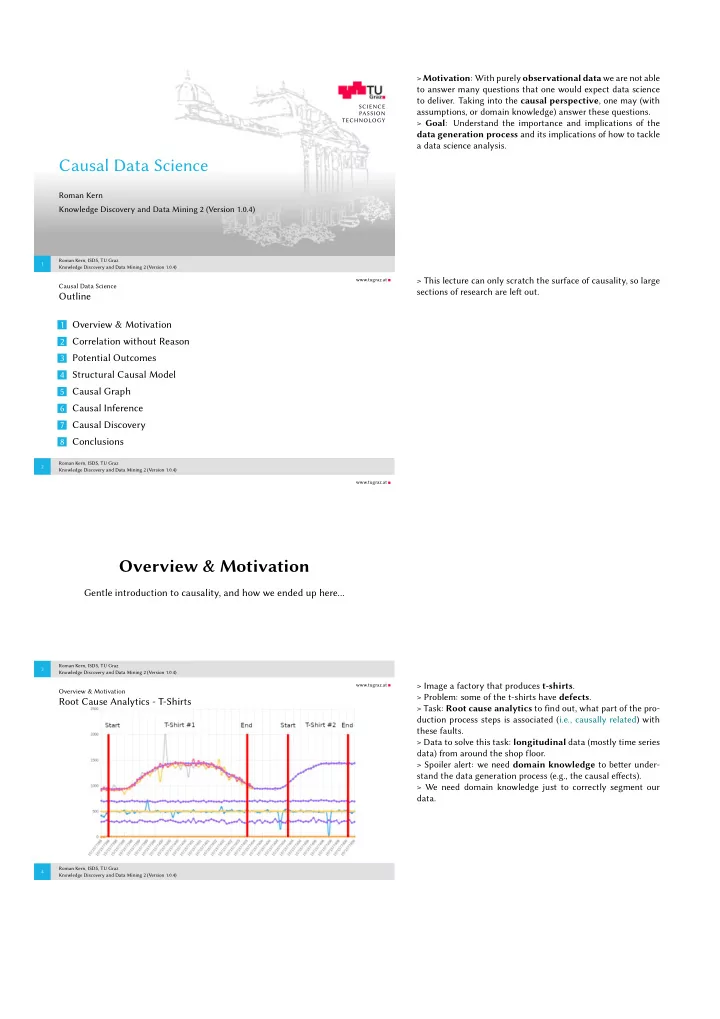
Simpson’s Paradox Recall Covid’19 case

A - age, C - country, CRF - case fatality rate A C CFR Age (A) is a confounder A C CFR Age (A) is a mediator We assumed age to be a mediator → CFR is higher in Italy (and the total causal effect (TCE) is the difference in CFRs).

Roman Kern, ISDS, TU Graz Knowledge Discovery and Data Mining 2 (Version 1.0.4) 73

> Here the intervention can be seen as change the country from China (no treatment) to Italy (treatment). > What is the correct question if we want to find out: what is the effect of the country (Italy) on CFR? > Possible questions: > - What is the average effect of the country? (mediator) > - What is the age group effect of the country? (confounder) > In our case we assume age to be the mediator, as Italy causes people to get old → we now know, which is the right question to ask.

www.tugraz.at

Causal Inference

Causal Effects Total causal effect (TCE)

“What would be the effect on mortality of changing the country from China to Italy?”

Controlled direct effect (CDE)

“For 50–59 year-olds, is it safer to get the disease in China or in Italy?” Controlling for a value of the mediator (i.e., different for each age group)

Natural direct effect (NDE)

“For the Chinese case demographic, would the Italian approach have been beter?”

Natural indirect effect (NIE)

“How would the overall CFR in China change if the case demographic had instead been that from Italy, while keeping all else (i.e., the CFR’s of each age group) the same?”

Roman Kern, ISDS, TU Graz Knowledge Discovery and Data Mining 2 (Version 1.0.4) 74

> Measuring the causal effect in various ways to learn about the causal implications. > Mediation analysis to split the total causal effect into direct and indirect effect. > Real world scenarios it is ofen difficult or even impossible to control both the treatment and the mediator > Much more, e.g. Sample Average Treatment Effect (SATE), Population Average Treatment Effect (PATE), Population Aver- age Treatment Effect for the Treated (PATT), Conditional Aver- age Treatment Effect, ... > For mediation analysis also see: https://david-salazar.

github.io/2020/08/26/causality-mediation-analysis/

www.tugraz.at

Causal Inference

Causal Effects

Roman Kern, ISDS, TU Graz Knowledge Discovery and Data Mining 2 (Version 1.0.4) 75

Evolution of TCE, NDE, and NIE of changing country from China to Italy on total CFR over time. We com- pare static data from China [27] with different snapshots from Italy reported by [10]. The direct effect initially was negative, meaning that age-specific mortality in Italy was lower; however, it changes sign around mid-March when an overloaded health system in northern Italy was re- ported [1]. The indirect effect remains mostly constant at a substantial +3–3.5%. > von Kügelgen, J., Gresele, L. and Schölkopf, B. (2020) ‘Simpson’s paradox in Covid-19

case fatality rates: a mediation analysis of age-related causal effects’, pp. 10–19.

www.tugraz.at

Causal Inference

Simpson’s Paradox #2 Example: Kidney Stone Treatment Stone size vs Treatment Treatment A Treatment B Interpretation Small stones 93% (81/87) 87% (234/270) A > B Large stones 73% (192/263) 69% (55/80) A > B Both 78% (273/350) 83% (289/350) A < B

Patients, who suffer from kidney stones receive either treatment A or B, and then the success of the treatment is measured, for multiple patients then a success rate can be computed. We are interested to know: Which treatment is beter?

Roman Kern, ISDS, TU Graz Knowledge Discovery and Data Mining 2 (Version 1.0.4) 76

> Example taken from Wikipedia:

https://en.wikipedia.

• rg/wiki/Simpson’s_paradox

> There are two treatments (A, B) for kidney stones, where the stones have different sizes (small, large). > The outcome is the success rate of the treatment (in percent). > When conditioned on the stone size, treatment A appears to be beter than B (for both small and large stones), but in total the direction is reversed. > Note: The numbers in the brackets specify the size of the groups, where we can observe a skewed distribution (while there as many receiving the two treatments, in this case 350 patients for each treatment).

www.tugraz.at

Causal Inference

Simpson’s Paradox #2 Size Treatment Success

Stone size is a confounder, i.e., A > B

Size Treatment Success

Stone size is a mediator, i.e., A < B Since the doctors already assume treatment A to be beter, they assign more severe cases (i.e., larger stones) to treatment A (and less severe cases to treatment B) → the size of the stone has a causal effect on the treatment (stone size is a confounder), A > B.

Roman Kern, ISDS, TU Graz Knowledge Discovery and Data Mining 2 (Version 1.0.4) 77

> Crucially, the size has an influence on the outcome as well, in fact in this case we expect that the “influence” of the stone size if bigger than the influence of the treatment alone, known as Cornfield’s conditions: > P(success | small stone) − P(success | large stone) > P(success | treatment B) − P(success | treatment A) > In this case: 0.16 > 0.05 > Schield, M. and Milo Schield (1999) ‘Simpson’s paradox and cornfield’s conditions’, ASA Proceedings of the Section on Sta- tistical Education, 1999, pp. 106–111. > This is a classical example of bias in data science and we of- ten assume that the treatment to be randomised, while in prac- tice it ofen is not. > e.g., if the workers/engineers in the t-shirt manufacturing plant already assume a certain machine to provide beter/worse results, this may bias the results. > Practical problem of data science: how do we find these potential confounders?

www.tugraz.at

Causal Inference

Causal Inference - Summary We need to study the causal relationships Which we assume to be given (and correct) We study, which variables are observed (conditioned) We select the approach and derive the matching formula Finally, apply on the data

Roman Kern, ISDS, TU Graz Knowledge Discovery and Data Mining 2 (Version 1.0.4) 78

> In many case it may happen that we require binning. > Is is important that the bins are then sufficiently large, i.e., enough data points/instances available per bin.

www.tugraz.at

Causal Discovery

Given data, can we infer the causal model?

Roman Kern, ISDS, TU Graz Knowledge Discovery and Data Mining 2 (Version 1.0.4) 79 www.tugraz.at

Causal Discovery

Assumptions Sufficiency, there are no hidden confounders Markov assumption, an event is independent from non-descendants, if conditioned on its parents (Weak) faithfulness, there might observe a correlation if there is a causal relationships Faithfulness, there expect to observe a correlation if there is a causal relationships

Roman Kern, ISDS, TU Graz Knowledge Discovery and Data Mining 2 (Version 1.0.4) 80

> Ofen, faithfulness is required, because, if due to spurious rea- sons we do not observe a correlation, even if the data generation process (causality) may indicate so, there is litle chance to suc- cessfully recover the correct causal structure.

www.tugraz.at

Causal Discovery

Additive Noise Model Recall SCM Yi = fi(Xi, Ui) For the Additive Noise Model (ANM) we assume Yi = fi(Xi) + Ui, assuming, Xi ⊥

⊥ Ui

Roman Kern, ISDS, TU Graz Knowledge Discovery and Data Mining 2 (Version 1.0.4) 81 www.tugraz.at

Causal Discovery

Additive Noise Model We further assume a non-linear function and a “bounded” noise

→ expect the noise on Y to be independent from X

While, vice-versa, do not expect this behaviour

Roman Kern, ISDS, TU Graz Knowledge Discovery and Data Mining 2 (Version 1.0.4) 82

> Image taken from: Lopez-Paz, D. et al. (2017) ‘Discovering causal signals in images’, Proceedings - 30th IEEE Conference

• n Computer Vision and Patern Recognition, CVPR 2017, 2017-

Janua, pp. 58–66. doi: 10.1109/CVPR.2017.14..

www.tugraz.at

Causal Discovery

Additive Noise Model Application Regress Y on X Non-linear, good-fit Compute residuals E If X and E are not independent, then X causes Y

Roman Kern, ISDS, TU Graz Knowledge Discovery and Data Mining 2 (Version 1.0.4) 83 www.tugraz.at

Causal Discovery

Granger Causality Identify causal relationships in multivariate time series Intuition If Xi is uniquely helpful to predict future values of Xj, in the presence of other predictive time series Xk (may be multiple) ... then we assume Xi → Xj, i.e., Xi forecasts Xj Conditional ignorability assumption is not satisfied

→ assumes no hidden confounders

e.g., for stock market prediction need to know influence of other stocks, economy, ...

Roman Kern, ISDS, TU Graz Knowledge Discovery and Data Mining 2 (Version 1.0.4) 84

> Extended intuition: ablation study to single out the predictive power of Xi on Xj > e.g., compare prediction using P(Xj | Xk) vs P(Xj | Xk, Xi) > Qote: “it cannot be used to discover real causality”, as “the values of both treatment variable X and control variable Y maybe driven by a third variable” > Tsapeli, F., Musolesi, M. and Tino, P. (2017) ‘Non-parametric causality detection: An application to social media and finan- cial data’, Physica A: Statistical Mechanics and its Applications. Elsevier B.V., 483, pp. 139–155. doi: 10.1016/j.physa.2017.04.101. > “Transfer entropy is a model-free equivalent of Granger causality.” > Does not detect causality, but mere temporally related phe- nomena.

www.tugraz.at

Causal Discovery

Granger Causality Typically solved via (linear) regression Individual coefficients for lagged causality i.e., The causal relationship may manifest itself only afer some

• bservations

Roman Kern, ISDS, TU Graz Knowledge Discovery and Data Mining 2 (Version 1.0.4) 85

> The lag is typically assumed to be constant and independent from other factors. > Another typical assumption is stationarity of the time series.

www.tugraz.at

Conclusions

Practical Aspects and Conclusion

Roman Kern, ISDS, TU Graz Knowledge Discovery and Data Mining 2 (Version 1.0.4) 86 www.tugraz.at

Conclusions

Causal Data Science Process Gain an understanding of the domain e.g., causal graph, what happens when, five whys, Ishikawa diagram, FMEA Gain an understaning of the data e.g., correlation anlaysis, visual tools, dimensionality reduction, EDA Formulate questions/hypothesis Find answers (by following the causal pathways) Iterate! (e.g., refine questions, gather more data)

Roman Kern, ISDS, TU Graz Knowledge Discovery and Data Mining 2 (Version 1.0.4) 87 www.tugraz.at

Conclusions

Causal Data Science Process Best practice Check, if the causal relationships (from the domain expert) hold true in the data (faithfulness) Collect constraints not available as causal relationship Keep held-out data to validate findings If possible, run controlled experiments to experimentally validate findings Be aware of assumptions and their implications

Roman Kern, ISDS, TU Graz Knowledge Discovery and Data Mining 2 (Version 1.0.4) 88

www.tugraz.at

Conclusions

Practical Aspects Confounders Unobserved confounding nonetheless remains a major obstacle in practice

→ include more data (more variables) into the dataset

Roman Kern, ISDS, TU Graz Knowledge Discovery and Data Mining 2 (Version 1.0.4) 89

> https://fairmlbook.org/causal.html.

www.tugraz.at

Conclusions

Practical Aspects Building causal graphs is not trivial3 Important: the causal graph is the statistical, causal interpretation

• f the underlying data generation process

When to merge/split nodes? What confounders realistically exists? Which can be simply ignore? Which causal relationships are transitive? Mediator vs. moderator?

3Even with domain knowledge

Roman Kern, ISDS, TU Graz Knowledge Discovery and Data Mining 2 (Version 1.0.4) 90

> The data scientist should draw the causal graph, not the do- main expert.

www.tugraz.at

Conclusions

Practical Aspects Split the event/variable into an unobservable and observable Ofen assumed a measurement equals the treatment T T ∗ Y T is the true treatment (not observed), T ∗ is a measurement (observed)

Roman Kern, ISDS, TU Graz Knowledge Discovery and Data Mining 2 (Version 1.0.4) 91 www.tugraz.at

Conclusions

Takeaway Message Causality is a powerful tool Guides the data scientist to ask the correct questions ... and to correctly answer them (e.g., unbiased) But, purely data-driven causal inference is not possible ... domain knowledge (e.g., via causal graphs) is always needed ... if not available, avoid jumping to (causal) conclusions

Roman Kern, ISDS, TU Graz Knowledge Discovery and Data Mining 2 (Version 1.0.4) 92

www.tugraz.at

Conclusions

The End

Thank you for your atention!

Roman Kern, ISDS, TU Graz Knowledge Discovery and Data Mining 2 (Version 1.0.4) 93