Bounding Deviation from Expectation Theorem [Markov Inequality] For - - PowerPoint PPT Presentation

Bounding Deviation from Expectation

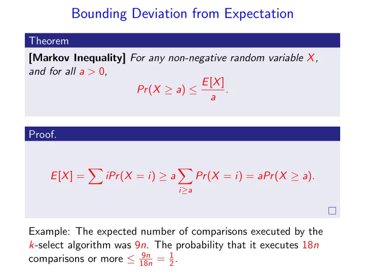
Theorem [Markov Inequality] For any non-negative random variable X, and for all a > 0, Pr(X ≥ a) ≤ E[X] a . Proof. E[X] =

• iPr(X = i) ≥ a
• i≥a

Pr(X = i) = aPr(X ≥ a). Example: The expected number of comparisons executed by the k-select algorithm was 9n. The probability that it executes 18n comparisons or more ≤ 9n

18n = 1 2.

Variance

Definition The variance of a random variable X is Var[X] = E[(X − E[X])2] = E[X 2] − (E[X])2. Definition The standard deviation of a random variable X is σ(X) =

• Var[X].

Chebyshev’s Inequality

Theorem For any random variable X, and any a > 0, Pr(|X − E[X]| ≥ a) ≤ Var[X] a2 . Proof. Pr(|X − E[X]| ≥ a) = Pr((X − E[X])2 ≥ a2) By Markov inequality Pr((X − E[X])2 ≥ a2) ≤ E[(X − E[X])2] a2 = Var[X] a2

Theorem For any random variable X and any a > 0: Pr(|X − E[X]| ≥ aσ[X]) ≤ 1 a2 . Theorem For any random variable X and any ε > 0: Pr(|X − E[X]| ≥ εE[X]) ≤ Var[X] ε2(E[X])2 .

Theorem If X and Y are independent random variables E[XY ] = E[X] · E[Y ]. Proof. E[XY ] =

• i
• j

i · jPr((X = i) ∩ (Y = j)) =

• i
• j

ijPr(X = i) · Pr(Y = j) =

• i

iPr(X = i)  

j

jPr(Y = j)   .

Theorem If X and Y are independent random variables Var[X + Y ] = Var[X] + Var[Y ]. Proof. Var[X + Y ] = E[(X + Y − E[X] − E[Y ])2] = E[(X − E[X])2 + (Y − E[Y ])2 + 2(X − E[X])(Y − E[Y ])] = Var[X] + Var[Y ] + 2E[X − E[X]]E[Y − E[Y ]] Since the random variables X − E[X] and Y − E[Y ] are independent. But E[X − E[X]] = E[X] − E[X] = 0.

Bernoulli Trial

Let X be a 0-1 random variable such that Pr(X = 1) = p, Pr(X = 0) = 1 − p. E[X] = 1 · p + 0 · (1 − p) = p. Var[X] = p(1 − p)2 + (1 − p)(0 − p)2 = p(1 − p)(1 − p + p) = p(1 − p).

A Binomial Random variable

Consider a sequence of n independent Bernoulli trials X1, ...., Xn. Let X =

n

• i=1

Xi. X has a Binomial distribution X ∼ B(n, p). Pr(X = k) = n k

• pk(1 − p)n−k.

E[X] = np. Var[X] = np(1 − p).

The Geometric Distribution

• How many times do we need to perform a trial with

probability p for success till we get the first success?

• How many times do we need to roll a dice until we get the

first 6? Definition A geometric random variable X with parameter p is given by the following probability distribution on n = 1, 2, . . .. Pr(X = n) = (1 − p)n−1p.

Memoryless Distribution

Lemma For a geometric random variable with parameter p and n > 0, Pr(X = n + k | X > k) = Pr(X = n). Proof. Pr(X = n + k | X > k) = Pr((X = n + k) ∩ (X > k)) Pr(X > k) = Pr(X = n + k) Pr(X > k) = (1 − p)n+k−1p ∞

i=k(1 − p)ip

= (1 − p)n+k−1p (1 − p)k = (1 − p)n−1p = Pr(X = n).

Conditional Expectation

Definition E[Y | Z = z] =

• y

y Pr(Y = y | Z = z), where the summation is over all y in the range of Y .

Lemma For any random variables X and Y , E[X] = Ey[EX[X | Y ]] =

• y

Pr(Y = y)E[X | Y = y], where the sum is over all values in the range of Y . Proof.

• y

Pr(Y = y)E[X | Y = y] =

• y

Pr(Y = y)

• x

x Pr(X = x | Y = y) =

• x
• y

x Pr(X = x | Y = y) Pr(Y = y) =

• x
• y

x Pr(X = x ∩ Y = y) =

• x

x Pr(X = x) = E[X].

Example

Consider a two phase game:

• Phase I: roll one die. Let X be the outcome.
• Phase II: Flip X fair coins, let Y be the number of HEADs.
• You receive a dollar for each HEAD.

Y is distributed B(X, 1

2),

E[Y | X = a] = a 2 E[Y ] =

6

• i=1

E[Y | X = i]Pr(X = i) =

6

• i=1

i 2Pr(X = i) = 7 4

Geometric Random Variable: Expectation

• Let X be a geometric random variable with parameter p.
• Let Y = 1 if the first trail is a success, Y = 0 otherwise.
• E[X]

= Pr(Y = 0)E[X | Y = 0] + Pr(Y = 1)E[X | Y = 1] = (1 − p)E[X | Y = 0] + pE[X | Y = 1].

• If Y = 0 let Z be the number of trials after the first one.
• E[X] = (1 − p)E[Z + 1] + p · 1 = (1 − p)E[Z] + 1
• But E[Z] = E[X], giving E[X] = 1/p.

Variance of a Geometric Random Variable

• We use

Var[X] = E[(X − E[X])2] = E[X 2] − (E[X])2.

• To compute E[X 2], let Y = 1 if the first trial is a success,

Y = 0 otherwise.

• E[X 2]

= Pr(Y = 0)E[X 2 | Y = 0] + Pr(Y = 1)E[X 2 | Y = 1] = (1 − p)E[X 2 | Y = 0] + pE[X 2 | Y = 1].

• If Y = 0 let Z be the number of trials after the first one.
• E[X 2]

= (1 − p)E[(Z + 1)2] + p · 1 = (1 − p)E[Z 2] + 2(1 − p)E[Z] + 1,

• E[Z] = 1/p and E[Z 2] = E[X 2].
• E[X 2]

= (1 − p)E[(Z + 1)2] + p · 1 = (1 − p)E[Z 2] + 2(1 − p)E[Z] + 1,

• E[X 2] = (1−p)E[X 2]+2(1−p)/p+1 = (1−p)E[X 2]+(2−p)/p,
• E[X 2] = (2 − p)/p2.

Variance of a Geometric Random Variable

Var[X] = E[X 2] − E[X]2 = 2 − p p2 − 1 p2 = 1 − p p2 .

Back to the k-select Algorithm

• Let X be the total number of comparisons.
• Let Ti be the number of iterations between the i-th successful

call (included) and the i + 1-th (excluded):

• X ≤ log3/2 n

i=0

n(2/3)iTi.

• Ti ∼ G(1/3), therefore E[Ti] = 3, Var[Ti] = 9/4.
• Expected number of comparisons:

E[X] ≤ log3/2 n

j=0

3n (2/3)j ≤ 9n.

• Variance of the number of comparisons:

Var[X] = log3/2 n

i=0

n2(2/3)2iVar[Ti] ≤ 11n2 Pr(|X − E[X]| ≥ δE[X]) ≤ Var[X] δ2E[X]2 ≤ 11n2 δ281n2

Example: Coupon Collector’s Problem

Suppose that each box of cereal contains a random coupon from a set of n different coupons. How many boxes of cereal do you need to buy before you obtain at least one of every type of coupon? Let X be the number of boxes bought until at least one of every type of coupon is obtained. Let Xi be the number of boxes bought while you had exactly i − 1 different coupons. X =

n

• i=1

Xi Xi is a geometric random variable with parameter pi = 1 − i − 1 n .

E[Xi] = 1 pi = n n − i + 1. E[X] = E n

• i=1

Xi

• =

n

• i=1

E[Xi] =

n

• i=1

n n − i + 1 = n

n

• i=1

1 i = n ln n + Θ(n).

Example: Coupon Collector’s Problem

• We place balls independently and uniformly at random in n

boxes.

• Let X be the number of balls placed until all boxes are not

empty.

• What is E[X]?

• Let Xi = number of balls placed when there were exactly i − 1

non-empty boxes.

• X = n

i=1 Xi.

• Xi is a geometric random variable with parameter

pi = 1 − i−1

n .

• E[Xi] = 1

pi = n n − i + 1. E[X] = E n

• i=1

Xi

• =

n

• i=1

E[Xi] =

n

• i=1

n n − i + 1 = n

n

• i=1

1 i = n ln n + Θ(n).

Back to the Coupon Collector’s Problem

• Suppose that each box of cereal contains a random coupon

from a set of n different coupons.

• Let X be the number of boxes bought until at least one of

every type of coupon is obtained.

• E[X] = nHn = n ln n + Θ(n)
• What is Pr(X ≥ 2E[X])?
• Applying Markov’s inequality

Pr(X ≥ 2nHn) ≤ 1 2.

• Can we do better?

• Let Xi be the number of boxes bought while you had exactly

i − 1 different coupons.

• X = n

i=1 Xi.

• Xi is a geometric random variable with parameter

pi = 1 − i−1

n .

• Var[Xi] ≤ 1

p2 ≤ ( n n−i+1)2.

• Var[X] =

n

• i=1

Var[Xi] ≤

n

• i=1
• n

n − i + 1 2 = n2

n

• i=1

1 i 2 ≤ π2n2 6 .

• By Chebyshev’s inequality

Pr(|X − nHn| ≥ nHn) ≤ n2π2/6 (nHn)2 = π2 6(Hn)2 = O

• 1

ln2 n

• .

Direct Bound

• The probability of not obtaining the i-th coupon after

n ln n + cn steps:

• 1 − 1

n n(ln n+c) ≤ e−(ln n+c) = 1 ecn.

• By a union bound, the probability that some coupon has not

been collected after n ln n + cn step is e−c.

• The probability that all coupons are not collected after 2n ln n

steps is at most 1/n.