Beta Decay Beta Decay Microscopic picture Microscopic picture On - - PDF document

Beta Decay Beta Decay

Microscopic picture Microscopic picture

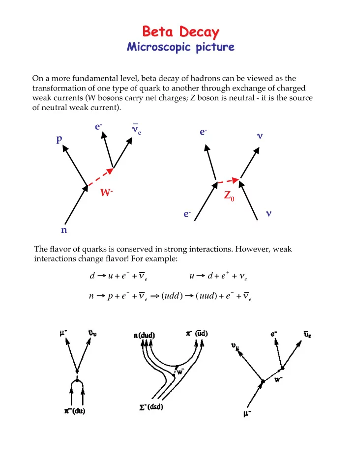
On a more fundamental level, beta decay of hadrons can be viewed as the transformation of one type of quark to another through exchange of charged weak currents (W bosons carry net charges; Z boson is neutral - it is the source

• f neutral weak current).

n p e- νe _ W- e- ν e- ν Z0

The flavor of quarks is conserved in strong interactions. However, weak interactions change flavor! For example:

u d + e

+ + e

d u + e

+ e

n p + e

+ e (udd) (uud) + e + e

Beta Decay Beta Decay

Microscopic picture Microscopic picture

When a quark decays, the new quark does not have a definite flavor. For instance:

u d'= d cosc + ssinc

Cabibbo angle

However, the observed weak transitions are between quarks of definite

• flavor. The strong-interaction quark eigenstates

d' s' b'

• =

U ud U us U ub U cd U cs U cb U td U ts U tb

• d

s b

• This means that the observed beta-decay strength in reactions is modified by

the mixing angle.

u d

• c

s

• t

b

• u

d'

• c

s'

• t

b'

• are different from weak interaction eigenstates).

Cabibbo _Kobayashi- Maskawa (CKM) matrix

For nuclear beta-decay, we are mainly concerned with the transition between u- and d-quarks. As a result, only the product enters into the process.

GV = GF cosc

Beta Decay Beta Decay

Microscopic picture Microscopic picture

What are the consequences of parity violation in beta decay?

h = r r p p

helicity

The eigenvalue of h is v/c. For a massless particle, the eigenvalues of h can be only +1 or -1. In general, the particle with

• h>0 is called “right-handed”
• h<0 is called “left-handed”

Experimentally,

h( e) 1 , h( e) +1 , h(e

±) = mv/c

All the leptons emitted in beta-decays are left-handed and all antileptons - right-handed!

The operators that are scalars, pseudoscalars and tensors produce leptons of both helicities under a parity transformation. Only vector operators V and axial vector operators A can accommodate the observed result. Furthermore, since V and A are of different parity, they must appear in a linear combination. This leads to the V-A theory of beta decay. In principle, both V and A parts should be characterized by different coupling constants, GV and GA, respectively. The vector current is known to be a conserved quantity (CVC hypothesis)

V

, = 0

four-divergence

For the axial vector current, there is not such a relation. The four-divergence

• f A (a pseudoscalar!) does not vanish. The pion is a pseudoscalar particle. Hence

the weak interaction is modified in the presence of strong interactions. This leads to a partially conserved axial-vector current (PCAC) hypothesis:

A, = a

a constant the pion field

Beta Decay Beta Decay

Microscopic picture (cont.) Microscopic picture (cont.)

How to relate GV and GA?

gA GA GV = f gn MNc

2

pion decay constant pion-nucleon coupling constant Goldberger-Trieman relation

Experimentally, gA=-1.259

This value is close to obtained from the relation above. It is a nice confirmation of the PCAC gA 1.31

Matrix elements Matrix elements

Vint g r r

n r

r

p

( ) r

r

n r

r

e

( ) r

r

n r

r

• (

) ˆ

O (n p)

zero-range

The nuclear operator transforming a neutron into a proton must be one body in nature. Hence it must involve the isospin raising or lowering operators. In the non-relativistic limit, the vector part may be represented by the unity

• perator times and the axial-vector part by a product of and σ. (A

proper derivation requires manipulation with Dirac 4-component fuctions and γ matrices!)

± ±

Vint GV ±( j) + gA r

• ( j) r

(j)

[ ]

j=1 A

• Fermi decay, carries

zero angular momentum Gamow-Teller decay, carries one unit of angular momentum

Beta Decay Beta Decay

Allowed decays Allowed decays Fermi transitions Fermi transitions

J f M fTfT0 f Tm JiMiTiT0i = Ti(Ti +1) T0i(T0i m1)Ji J fM i M fTiT fT0i m1T0 f

In reality, isospin is violated by the electromagnetic force, but the violation is weak.

J f = Ji J = 0

( )

Tf = Ti 0 T = 0, but Ti = 0 Tf = 0 forbidden

( )

T0 f = T0i m1 T0 =1

( )

= 0 no parity change

T+ has rank unity!

Gamow Gamow-Teller transitions

• Teller transitions

The matrix element strongly depends on the structure of the wave function!

J = 0,1 but Ji = 0 J f = 0 forbidden T = 0,1 but Ti = 0 Tf = 0 forbidden T0 f = T0i m1 T0 =1

( )

= 0 no parity change

The absolute values of GT matrix elements are generally smaller than those for Fermi transitions.

fT = const F

2 + gA 2 GT 2 squared matrix elements

Beta Decay Beta Decay

Forbidden transitions Forbidden transitions

Forbidden transitions involve parity change and a spin change of more than

• ne unit. They come from the higher-order terms in the expansion of electron

and neutrino plane waves into spherical harmonics. Forbidden decays are classified into different groups by the L-value of the spherical harmonics

• involved. The selection rules for the Lth-order forbidden transitions are:

J = L or L ±1, = (1)

L

Experimental log fT values

Beta Decay Beta Decay

electron capture processes electron capture processes

Electron capture leads to a vacancy being created in one of the strongest bound atomic states, and secondary processes are observed such as the emission of X- rays and Auger electrons. Auger electrons are electrons emitted from one of the

• uter electron shells and take away some of the remaining energy.

Capture is most likely for a 1s-state electron. The K-electron wave function at the origin is maximal and is given by

e (0) = 1

• Zmee2

h

2

• 3/2

W

EC = Ev 2 Mfi ' 2g 2

• 2h

4c 3

Zmee2 h

2

• 3

The electron capture probability is thus given by: