Basics of HMMs You should be able to take this and fill in the - PDF document

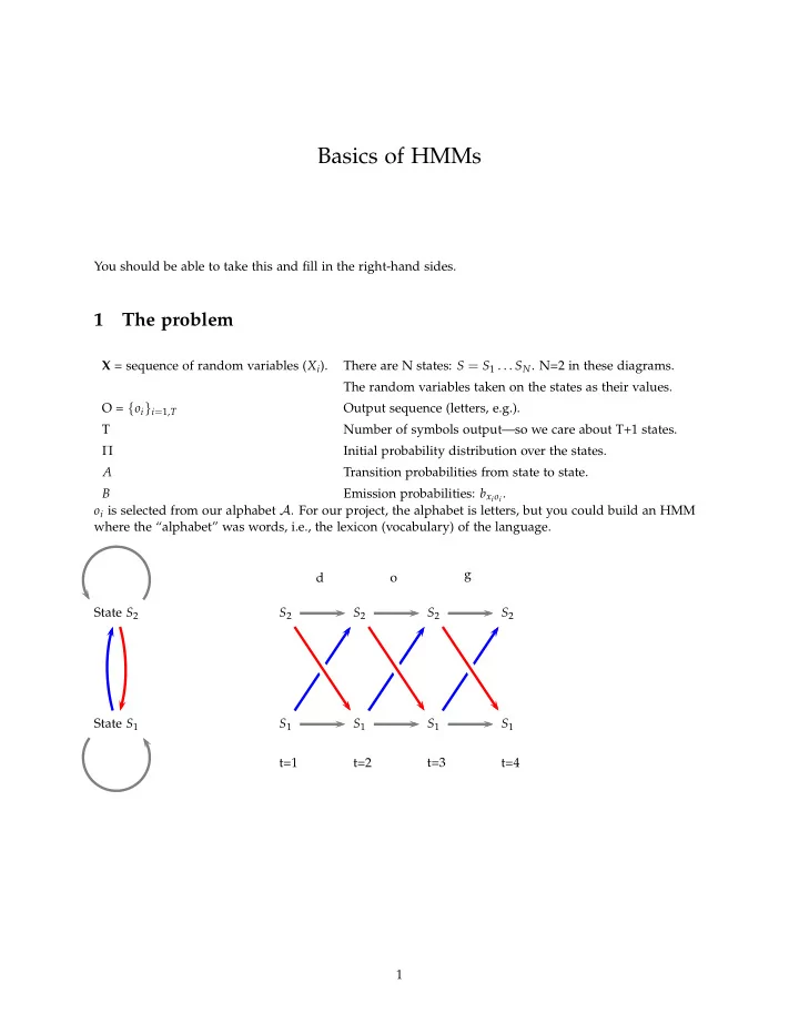
Basics of HMMs You should be able to take this and fill in the right-hand sides. 1 The problem X = sequence of random variables ( X i ). There are N states: S = S 1 . . . S N . N=2 in these diagrams. The random variables taken on the states as their values. O = { o i } i = 1, T Output sequence (letters, e.g.). T Number of symbols output—so we care about T+1 states. Π Initial probability distribution over the states. A Transition probabilities from state to state. B Emission probabilities: b x i o i . o i is selected from our alphabet A . For our project, the alphabet is letters, but you could build an HMM where the “alphabet” was words, i.e., the lexicon (vocabulary) of the language. g d o State S 2 S 2 S 2 S 2 S 2 State S 1 S 1 S 1 S 1 S 1 t=1 t=2 t=3 t=4 1

1 THE PROBLEM a 2,2 a 2,2 a 2,2 State S 2 S 2 S 2 S 2 a 2,1 a 2,1 π 2 π 1 a 1,2 = 1 − a 1,1 a 2,1 = 1 − a 2,2 a 1,2 a 1,2 State S 1 S 1 S 1 S 1 a 1,1 a 1,1 a 1,1 Markov model on states: limited lookback (horizon) : p ( X t + 1 = s i | X 1 . . . X t ) = p ( X t + 1 = s i | X t ) (1) Stationary p ( X t + 1 = s i | X t ) = p ( X 2 = s j | X 1 ) (2) = Transition matrix: a ij (3) So for fixed i , | S | ∑ a ij = j = 1 We initialize p ( X 1 ) = π i . So (what are we summing over?) ∑ π i = a 2,2 a 2,2 S 2 S 2 S 2 a 2,1 a 2,1 start a 1,2 a 1,2 S 1 S 1 S 1 a 1,1 a 1,1 2

2 THE VITERBI SEARCH FOR THE BEST PATH Now, X is a path , a sequence of states, such as X 1 X 2 X 2 . a 2,2 a 2,2 S 2 S 2 S 2 a 2,1 a 2,1 π 2 initial distribution a 1,2 a 1,2 π 1 S 1 S 1 S 1 a 1,1 a 1,1 T ∏ p ( X ) = p ( X 1 . . . X T ) = π x 1 a x i x i + 1 (4) i = 1 The probability of taking a path X and generating a string O is equal to the product of the probability of the path times the probability of emitting the correct letter at each point on the path. The probability of emitting the correct letter at each point on the path, given the path , is ∏ N t = 1 b x t o t b 2, o 2 S 2 S 2 S 2 b 1, o 1 S 1 S 1 S 1 2 The Viterbi search for the best path We often use µ to refer to the family of parameters. Find X to maximize p( X |O, µ ) or p( X ,O| µ ). We are searching over all paths of length exactly t-1 , not t . Let’s fix our ideas (as they say) by looking at a 2-state HMM, where the initial distribution π is uniform, and the states generate p,t,a,i with the following probabilities: 1 2 p .375 .125 t .375 .125 a .125 .375 i .125 .375 3

2 THE VITERBI SEARCH FOR THE BEST PATH From: To: 1 2 1 .25 .75 2 .75 .25 Here are two paths, the blue and the gray, out of the 32 paths through this lattice: S 2 S 2 S 2 S 2 S 2 S 1 S 1 S 1 S 1 S 1 t=1 t=2 t=3 t=4 t=5 What is the joint probability of each of those paths and the output tipa ? The blue path (disregarding the string emitted) has probability 0.5 × 0.75 × 0.75 × 0.75 × 0.75 = 3 4 2 9 = 81 512 . Its probability of emitting the sequence tipa is 3 4 81 6561 8 4 = 4096 , so the joint probability is 2097152 = .003 128. And how about the green path? It has probability 0.5 × 0.25 3 × 0.75 = 3 512 . Its probability of emitting the sequence tipa is 0.375 × 0.125 3 = 3 3 9 9 8 4 = 4096 = 0.000 732, so the joint probability is 2 21 = 2097152 = 0.000 004 291. But we really don’t want to do all those calculations for each path. δ j ( t ) = argmax X 1 ... X t − 1 P ( X 1 . . . X t − 1 , o 1 . . . o t − 1 , X t = j | µ ) (5) Initialize, for all states i : δ i ( 1 ) = (6) π i Induction: δ i ( t + 1 ) = max j δ j ( t ) a ji b jo t (7) Store backtrace: ψ j ( t + 1 ) = argmax i δ i ( t ) a ij b io t (8) Termination: ˆ X T + 1 = argmax i δ i ( T + 1 ) (9) Back trace: ˆ = X t + 1 ( t + 1 ) X t ψ ˆ (10) P ( ˆ X ) = max i δ i ( T + 1 ) (11) (12) 4

3 PROBABILITY OF A STRING, GIVEN CURRENT PARAMETERS 3 Probability of a string, given current parameters Given π , A , B , calculate p ( O | µ ) . How? It is the sum over all of the paths, of the probability of emitting O times the probability of that path. We call this a sum of joint path-string probabilities, each of which is p ( X ) ∏ T t = 1 b x t o t . This sum, then, is: T ∑ ∏ p ( X ) b x t o t (13) all paths X t = 1 N N ∑ ∏ ∏ π x 1 a a xtxt + 1 b x t o t (14) all paths X t = 1 t = 1 To paraphrase this: the probability of the string O is equal to the sum of the joint path-string probabilities. And each path-string probability is the product of exactly T transitional probabilities, T emission probabilities, and one initial ( π ) probability. We will return to this. α 2 ( 2 ) = α 2 ( 1 ) × a 2,2 × b 2, o 1 + α 1 ( 1 ) × a 1,2 × b 1, o 1 α 2 ( 0 ) α 2 ( 1 ) α 2 ( 2 ) S 2 S 2 S 2 X 2 S 1 S 1 S 1 X 1 α 1 ( 0 ) α 1 ( 1 ) α 1 ( 2 ) t=1 t=2 t=3 t=4 α 1 ( 2 ) = α 2 ( 1 ) × a 2,1 × b 2, o 1 + α 1 ( 1 ) × a 1,1 × b 1, o 1 Let’s calculate the probability of being at state i at time t , after emitting t-1 letters. This amounts to summing over all the paths only the first part of the path-string probability. That sum of products is the forward quantity α . The part that is left over (the sum over all the path-strings to the right of t ) will be summarized with the backward quantityt β . Forward: α i ( t ) = p ( X t = i , o 1 o 2 . . . o t − 1 | µ ) (15) Calculate : Initialize, for all states i : α i ( 1 ) = π i (16) = ∑ Induction: α i ( t + 1 ) α j ( t ) a ji b jo t (17) j = ∑ α i ( T + 1 ) End (total): P ( O | µ ) (18) (19) 5

3 PROBABILITY OF A STRING, GIVEN CURRENT PARAMETERS α 2 ( 0 ) α 2 ( 1 ) α 2 ( 2 ) α 2 ( 3 ) X 2 X 2 X 2 X 2 X 1 X 1 X 1 X 1 α 1 ( 0 ) α 1 ( 1 ) α 1 ( 2 ) α 1 ( 3 ) t=1 t=2 t=3 t=4 Similarly, we calculate the probability of generating the rest of the observed letters, given that we are at state i at time t . Backward: β i ( t ) = p ( o t . . . o T | X t = i , µ ) (20) Calculate : Initialize, for all states i : β i ( T + 1 ) = 1 (21) = ∑ Induction: β i ( t ) β j ( t + 1 ) a ij b io t (22) j = ∑ End (total): P ( O | µ ) π i β i ( 1 ) (23) i (24) β 2 ( 2 ) = β 1 ( 3 ) × a 2,2 × b 2, o 2 + β 2 ( 3 ) × a 2,1 × b 2, o 2 β 2 ( 0 ) β 2 ( 1 ) β 2 ( 2 ) β 2 ( 3 ) X 2 X 2 X 2 X 2 X 1 X 1 X 1 X 1 β 1 ( 0 ) β 1 ( 1 ) β 1 ( 2 ) β 1 ( 3 ) t=1 t=2 t=3 t=4 β 1 ( 2 ) = β 1 ( 3 ) × a 1,1 × b 1, o 1 + β 2 ( 3 ) × a 1,2 × b 1, o 1 6

3 PROBABILITY OF A STRING, GIVEN CURRENT PARAMETERS β 2 ( 0 ) β 2 ( 1 ) β 2 ( 2 ) β 2 ( 3 ) X 2 X 2 X 2 X 2 X 1 X 1 X 1 X 1 β 1 ( 0 ) β 1 ( 1 ) β 1 ( 2 ) β 1 ( 3 ) t=1 t=2 t=3 t=4 Mixing α and β : P ( O | µ ) = ∑ α i ( t ) β i ( t ) (25) i I think that you understand the whole idea if and only if you see that this equation is true. The basic insight is that the total probability of the string is equal to sum, over all paths through the lattice, of the product of the probability of the path times the probability of generating the string along that path. And that for any time t , we can partition all of those paths by looking at which set of paths goes through each of the states. If that is clear, then you have it. The probability that the HMM generates our string is equal to the sum of the joint path-string probability. Finding the best path through the HMM for a given set of data is the main reason we created the HMM. The state that the best path is in when it emits a given symbol is a label that the model assigns to that piece of data. In the case we look at, it is Consonant versus Vowel. The values of a are also very important for us. For a two-state model, there are two independent parameters, which we choose to be a 11 and a 22 . If we let the system learn from the data, and the data is linguistic letters, then both of those values should be low, because the system should learn a consonant/vowel distinction, and there is a strong tendency to alternative between C’s and V’s. 7

4 COUNTING EXPECTED (SOFT) COUNTS def Forward(States,Pi,thisword): Alpha= dict() for s in range(len(States)): Alpha[(s,1)] = Pi[s] for t in range(2,len(thisword)): for to_state in States: Alpha[(to_state,t)] = 0 for from_state in States: Alpha[(to_state,t)] += Alpha[(from_state,t-1)] * from_state.m_EmissionProbs[thisword[t]] * from_state.m_TransitionProbs[to_state] return Alpha def Backward( States, thisword): Beta = dict() last = len(thisword) + 1 for s in range(len(States)): Beta[(s, last)] = 1 for t in range(len(thisword),1,-1): for from_state in States: Beta[(from_state,t)] = 0 for to_state in States: Beta[(from_state,t)] += Beta[(to_state,t+1)] * from_state.m_EmissionProbs[thisword[t]] * from_state.m_Tra return Beta 4 Counting expected (soft) counts The probability of going from i → j from time t to time t + 1 during the generation of string O. Conceptually, this means looking at all the path-string pairs, and dividing them into N 2 different sets (based on which state they are in at time t and time t + 1). We know that the total probability of the string is the sum of a list of products, each with 2N+1 factors. For each pair i , j , we consider α i ( t ) a ij b io t β j ( t + 1 ) . What is the meaning of α i ( t ) a ij b io t β j ( t + 1 ) ? p ( O ) It is quite simply the proportion of the total probability (of the path-string pair) that goes through state i at t and state j at t + 1. And that is exactly what we mean by the expected count of the transitions between those two states at that time interval. And by construction, those N 2 soft counts add up to 1.0. p t ( i , j ) = p ( X t = i , X t + 1 = j | O , µ ) (26) p ( X t = i , X t + 1 = j , O | µ ) = (27) p ( O ) α i ( t ) a ij b io t β j ( t + 1 ) = (28) p ( O ) (29) 8