Basic Topics in PROLOG Practical matters Practical Matters Two - - PowerPoint PPT Presentation

Practical matters

Two Prologs are installed on the OSU Ling. Dept. UNIX machines:

• Sicstus:
• starting:

– at UNIX prompt: prolog – in Emacs: M-x run-prolog

• manual (652 pages – so don’t just print it!): links on course web page
• r ~dm/resources/manuals/sicstus/
• SWI-Prolog:
• starting: pl
• loading graphical tracer: ?- guitracer.
• manual: links on course web page or ~dm/resources/manuals/swi-prolog/

2

A brief reminder (2)

A PROLOG program consists of a set of Horn clauses:

• unit clauses (facts)

– Syntax: predicate followed by a dot – Example: father(tom,mary).

• non-unit clauses (rules)

– Syntax: rel0 :- rel1, ..., reln. – Example: grandfather(Old,Young) :- father(Old,Middle), father(Middle,Young).

Cases and Structural Induction 4

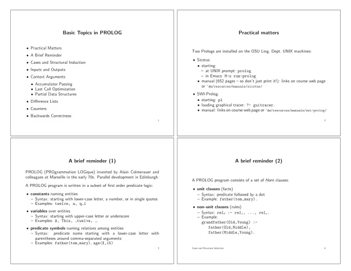
Basic Topics in PROLOG

• Practical Matters
• A Brief Reminder
• Cases and Structural Induction
• Inputs and Outputs
• Context Arguments
• Accumulator Passing
• Last Call Optimization
• Partial Data Structures
• Difference Lists
• Counters
• Backwards Correctness

1

A brief reminder (1)

PROLOG (PROgrammation LOGique) invented by Alain Colmerauer and colleagues at Marseille in the early 70s. Parallel development in Edinburgh. A PROLOG program is written in a subset of first order predicate logic:

• constants naming entities

– Syntax: starting with lower-case letter, a number, or in single quotes – Examples: twelve, a, q 1

• variables over entities

– Syntax: starting with upper-case letter or underscore – Examples: A, This, twelve,

• predicate symbols naming relations among entities

– Syntax: predicate name starting with a lower-case letter with parentheses around comma-separated arguments – Examples: father(tom,mary), age(X,15)

3

Compound terms as data structure for recursive relations

To define (interesting) recursive relations, one needs a richer data structure than the constants used so far: compound terms.

• A compound term comprises a functor and a sequence of one or more

terms, the argument. Atoms can be thought of as functors with arity 0.

• Compound terms are standardly written in prefix notation.

Example: bin tree(s, np, bin tree(vp,v,n)) Infix and postfix operators can also be defined, but need to be declared using op/3.

Cases and Structural Induction 6

Four equivalent representations: 1. .(a, .(b, .(c, .(d,[])))) 2. [a | [b | [c | [d | []]]]] 3. [a,b,c,d] 4. a b c d [] . . . .

Cases and Structural Induction 8

Basic use of arguments: Discriminate between cases

direction_adjective(north, boreal). direction_adjective(south, austral). direction_adjective(east, oriental). direction_adjective(west, occidental). abs_diff(X, Y, Diff) :- compare(R, X, Y), abs_diff(R, X, Y, Diff). abs_diff(<,X,Y,Diff) :- Diff is Y-X. abs_diff(>,X,Y,Diff) :- Diff is X-Y. abs_diff(=,_,_,0).

Cases and Structural Induction 5

Lists as special compound terms

Lists are represented as compound terms.

• empty list: represented by the atom “[]”
• non-empty lists: symbol ”.” as binary functor .(first,rest)

Example: .(a, .(b, .(c, .(d,[])))) Special notations:

• [ element1 | restlist ]

Example: [a | [b | [c | [d | []]]]]

• [ element1 , element2] = [ element1 | [element2 | []]]

Example: [a, b, c, d]

Cases and Structural Induction 7

arithmetic_value(-F, Value) :- % b2) recursive case arithmetic_value(F,Fval), Value is -Fval. arithmetic_value(E-F, Value) :- % b3) recursive case arithmetic_value(E,Eval), arithmetic_value(F,Fval), Value is Eval - Fval. arithmetic_value(E*F, Value) :- % b4) recursive case arithmetic_value(E,Eval), arithmetic_value(F,Fval), Value is Eval * Fval. arithmetic_value(E/F, Value) :- % b5) recursive case arithmetic_value(E,Eval), arithmetic_value(F,Fval), Value is Eval / Fval.

Cases and Structural Induction 10

A closer look at arguments: Inputs and Outputs

In principle, any argument (or part of it) can be input or output: birthday(byron, date(feb,4)). birthday(noelene, date(dec,25)). birthday(richard, date(oct,11)). birthday(clare, date(sep,15)). ?- birthday(byron,Date). ?- birthday(Person, date(feb,4)). ?- birthday(Person, date(feb,Day)).

Inputs and Outputs 12

Structural induction

is_list([]). % a) base/non-recursive case is_list([_|Tail]) :- % b) step/recursive/inductive case is_list(Tail). % arithmetic_value(Expr,Value) % is true when Expr represents an arithmetic expression and % Value is its numeric value arithmetic_value(c(N), N). % a) base case arithmetic_value(E+F, Value) :- % b1) recursive case arithmetic_value(E,Eval), arithmetic_value(F,Fval), Value is Eval + Fval.

Cases and Structural Induction 9

Why is this called structural induction?

• induction: defined recursively
• structural: recursion controlled by structure, not contents

Two things to watch out for:

• missing cases
• duplicate cases

An example for intentional duplicate cases: member(X,[X|_]). member(X,[_|L]) :- member(X,L).

Inputs and Outputs 11

Multiple output arguments

no output argument (true/false) greater_than(X,Y) :- X < Y.

• ne output argument: min

min(X, Y, X) :- X < Y. min(X, Y, Y) :- X >= Y. two output arguments: min, max min_and_max(X, Y, X, Y) :- X < Y. min_and_max(X, Y, Y, X) :- X >= Y.

Inputs and Outputs 14

Templates and meta-arguments

Template:

• Pattern for making/selecting things.
• Example: first argument of findall/3

?- findall(Month-Day, birthday(_Name,date(Month,Day)), Bag). Bag = [feb-4,dec-25,oct-11,sep-15] Meta-Argument:

• Term which stands for a goal.
• Example: argument of call/1 or second argument of findall/3

Inputs and Outputs 16

Predicates solving for particular arguments only

Built-in predicates involving arithmetic expressions

• Expression must be ground in evaluation of Answer is Expression

(expression has one value, but same value for infinitely many expressions)

• Both arguments must be ground in comparisons: E<F, E>F, E>=F, . . .

Predicates using these built-ins have specific inputs and outputs: factorial(0,1). factorial(N,N_Factorial) :- N > 0, M is N-1, factorial(M, M_Factorial), N_Factorial is M_Factorial*N. Recursive predicates often require particular arguments to terminate.

Inputs and Outputs 13

Order of arguments

Why a uniform ordering?

• clarity: consistency makes programs easier to understand
• efficiency: first argument indexing

Suggested ordering

• General rule: strict inputs < inputs-or-outputs < strict outputs
• Among strict inputs:

templates < meta-arguments < streams < selectors/indices < collections < other strict inputs

Inputs and Outputs 15

Selectors/Indices and Collections

Selectors/Indices:

• Terms which function like array subscripts.
• Example: first argument of arg/3

?- arg(3,p(a(n,o),b,c(m),d),X). X = c(m) ?- functor(p(a(n,o),b,c(m),d),Functor,Arity). Arity = 4, Functor = p Collections:

• essentially every compound term can be used as a collection
• Example: second argument of arg/3

Inputs and Outputs 18

The scope of variables

• There are no non-local variables in Prolog.
• Non-local variables are encoded as extra arguments of a predicate which

are passed unchanged into the recursion. % scale(SmallList,Multiplier,BigList) % True if each element of SmallList multiplied by Multiplier % is equal to the corresponding element of BigList. scale([], _, []). scale([X|Xs], Multiplier, [Y|Ys]) :- Y is X*Multiplier, scale(Xs, Multiplier, Ys).

Context Arguments: global variables as context 20

Streams

• Terms representing open files
• Example: third argument of open/3

file_write :-

• pen(myfile,write,MyStream), % modes: read/write/append

write(MyStream,’output to file’), write(’output to screen (standard output)’), close(MyStream). % simple case not using explicit streams simple_file_write :- tell(myfile), write(’output to file’), told.

Inputs and Outputs 17

Other ordering guidelines

• sequence order:

keep abstract sequences together (difference lists, accumulator pairs. . . )

• code/data consistency: e.g., Head < Tail since [Head|Tail]
• function direction: most general input first

Example: Term =.. List (every Term corresponds to a List, but not vice versa) ?- p(a(n,o),b,c(m),d) =.. List. X = [p,a(n,o),b,c(m),d] ?- Term =.. [1,a(n,o),b,c(m),d]. {TYPE ERROR: _169=..[1,a(n,o),b,c(m),d] - arg 2: expected atom, found 1}

Inputs and Outputs 19

Packaging contexts

context(conx(A,B,C,D),A,B,C,D). context_a(conx(A,_,_,_),A). context_b(conx(_,B,_,_),B). context_c(conx(_,_,C,_),C). context_d(conx(_,_,_,D),D). c(...) :- init(...,A,B,C,D,...), context(Context,A,B,C,D), p(...,Context,...), ...

Context Arguments: global variables as context 22

Accumulator passing

• There is no changing of variable values in Prolog.
• Two variables are used to store old and new value (accumulator passing).

len(List,Length) :- len(List, 0, Length). len([], N, N). len([_|L], N0, N) :- N1 is N0+1, len(L, N1, N).

Context Arguments: changing values as accumulator passing 24

% big_elements(FullList,SubList) % True if SubList is the list of those elements of % FullList which are bigger than 10, preserving order. big_elements(Input,Output) :- big_elements(Input, 10, Output). big_elements([], _, []). big_elements([Nbr|Nbrs], Bound, Bigs) :- Nbr < Bound, big_elements(Nbrs, Bound, Bigs). big_elements([Nbr|Nbrs], Bound, [Nbr|Bigs]) :- Nbr >= Bound, big_elements(Nbrs, Bound, Bigs).

Context Arguments: global variables as context 21

p(...,Context,...) :- ... context_a(Context,A), use_a(A), ... p(...,Context,...). p(...,Context,...) :- ... context_b(Context,B), use_b(B), ... p(...,Context,...).

Context Arguments: global variables as context 23

Multiple accumulator pairs

One changed in each recursion sum_pos_neg(List, Pos, Neg) :- sum_pos_neg(List, 0, Pos, 0, Neg). sum_pos_neg([], Pos, Pos, Neg, Neg). sum_pos_neg([X|Xs], Pos0, Pos, Neg0, Neg) :- X >= 0, Pos1 is Pos0+X, sum_pos_neg(Xs, Pos1, Pos, Neg0, Neg). sum_pos_neg([X|Xs], Pos0, Pos, Neg0, Neg) :- X < 0, Neg1 is Neg0+X, sum_pos_neg(Xs, Pos0, Pos, Neg1, Neg).

Context Arguments: changing values as accumulator passing 26

Last call optimization/Tail-recursion optimization

• Issue: Before execution can enter a recursive call, it has to save the

state of all variables.

• Idea: A recursive call as last goal in the body of a deterministic predicate

can be turned into a jump.

• Advantage: A jump does not require saving the state of the variables

before entering the recursion.

Context Arguments: last call optimization 28

rev(List, Reverse) :- rev(List, [], Reverse). rev([], Reverse, Reverse). rev([Head|Tail], Reverse0, Reverse) :- rev(Tail, [Head|Reverse0], Reverse).

Context Arguments: changing values as accumulator passing 25

Multiple accumulator pairs

Multiple changed in each recursion sum_and_ssq(List, Sum, SSQ) :- sum_and_ssq(List, 0, Sum, 0, SSQ). sum_and_ssq([], Sum, Sum, SSQ, SSQ). sum_and_ssq([X|Xs], Sum0, Sum, SSQ0, SSQ) :- Sum1 is Sum0 + X, SSQ1 is SSQ0+X, sum_and_ssq(Xs, Sum1, Sum, SSQ1, SSQ).

Context Arguments: changing values as accumulator passing 27

2 Call: slow len([b,c], M1)

• Prolog tries to match it against slow len([], 0), which fails.
• Prolog tries to match it against slow len([ |Tail2], N2), which

succeeds, binding Tail2=[c], N2=M1.

• A stack frame is created, holding N2 and M2.
• Prolog now has the goal slow len([c], M2 ).

3 Call: slow len([c], M2 )

• Prolog tries to match it against slow len([], 0), which fails.
• Prolog tries to match it against slow len([ |Tail3], N3), which

succeeds, binding Tail3=[], N3=M2.

• A stack frame is created, holding N3 and M3
• Prolog now has the goal slow len([],M3) .

30

1 Exit:

• Prolog returns to the first frame, and executes the goal N1 is M1+1,

which succeeds, binding N1=3, which binds X=3.

• The first stack frame is now released.

32

An example for ordinary recursion

slow_len([],0). slow_len([_|Tail],N) :- slow_len(Tail,M), N is M+1. How does the query slow len([a,b,c], X) work? 1 Call: slow len([a,b,c], X)

• Prolog tries to match it against slow len([],0), which fails.
• Prolog tries to match it against slow len([ |Tail1], N1), which

succeeds, binding Tail1=[b,c], N1=X.

• A stack frame is created, holding N1 and M1.
• Prolog now has the goal slow len([b,c], M1).

29

4 Call: slow len([], M3 )

• Prolog tries to match it against slow len([], 0), which succeeds,

binding M3=0. 3 Exit:

• Prolog returns to the third frame, and executes the goal N3 is M3+1,

which succeeds, binding N3=1.

• The third stack frame is now released.

2 Exit:

• Prolog returns to the second frame, and executes the goal N2 is M2+1, which

succeeds, binding N2=2.

• The second stack frame is now released.

31

lb Jump: N1 is N0+1 The goal N1 is NO+1 is executed, binding N1=1. 2a Jump: len([b,c], 1, X) The clause len([ |L], NO, N) is selected, binding L=[c], NO=1, N=X. 2b Jump: N1 is N0+1 Execution of the builtin goal binds N1=2. 3a Jump: len([c], 2, X) The clause len([ |L], NO, N) is selected, which binds L=[], NO=2, N=X. 3b Jump: N1 is NO+1 Execution of the builtin goal binds N1=3. 4 Jump: len([], 3, X) The clause len([], N, N) is selected, which binds X=3.

34

Classifying lists (an example for an accumulator pair)

is_proper_list(Term) :- classify_list(Term, proper, proper). is_partial_list(Term) :- classify_list(Term, proper, partial). is_a_list(Term) :- classify_list(Term, partial, partial). classify_list(V, _, X) :- var(V), !, X=partial. classify_list([],X,X). classify_list([_|T],X0,X) :- classify_list(T, X0, X).

Context Arguments: partial data structures 36

A tail-recursion example using the optimization

len(List,Length) :- len(List, 0, Length). len([], N, N). len([_|L], N0, N) :- N1 is N0+1, len(L, N1, N). How does the query len([a,b,c], X) work? 0 Call: len([a,b,c], X) Prolog tries to match it against len(List, Length), which succeeds, binding List=[a,b,c], Length=X. 1a Jump: len([a,b,c], 0, X) The clause len([ |L, NO, N) is selected, binding L=[b,c], N0=0, N=X.

33

Partial Data Structures

An instance i of a recursively defined data type t is referred to as

• proper if i is not a variable and each of its argument of type t is proper
• partial or incomplete otherwise.

Examples:

• proper lists: [], [_,_,_]
• partial lists: X, [a|_], [a|Rest]

Context Arguments: partial data structures 35

?- append([1,2],[3,4],X). % using "top-down" definition 1 1 Call: append([1,2],[3,4],_274) ? 2 2 Call: append([2],[3,4],_773) ? g Ancestors: 1 1 Call: append([1,2],[3,4],[1|_773]) 2 2 Call: append([2],[3,4],_773) ? 3 3 Call: append([],[3,4],_1938) ? g Ancestors: 1 1 Call: append([1,2],[3,4],[1,2|_1938]) 2 2 Call: append([2],[3,4],[2|_1938]) 3 3 Call: append([],[3,4],_1938) ? 3 3 Exit: append([],[3,4],[3,4]) ? 2 2 Exit: append([2],[3,4],[2,3,4]) ? 1 1 Exit: append([1,2],[3,4],[1,2,3,4]) ?

Context Arguments: partial data structures 38

Difference lists

• Idea: Carry around a partial data structure plus a reference to the holes

in it.

• Advantage: The partial data structure can be extended by filling a hole

with a (partial) data structure. Example: s(Phon0, Phon2) :- np(Phon0, Phon1), vp(Phon1, Phon2). np([john|Hole],Hole). np([laughs|Hole],Hole).

Difference Lists 40

Why use partial data structures?

Partial data structures allow building results top-down: append([], L, L). append([H|T], L, [H|R]) :- append(T,L,R). a bottom-up version (requires first argument is input): append([], L, L). append([H|T], L, X) :- append(T,L,R), X=[H|R].

Context Arguments: partial data structures 37

Walking through a tree vs. Unifying-in a pattern

path_data([], Tree, Datum) :- b_access(d, Tree, Datum). path_data([Arc|Arcs], Tree, Datum) :- b_access(Arc, Tree, Dtr), path_data(Arcs, Dtr, Datum). b_access(1, b(Lson,_,_), Lson). b_access(2, b(_,Rson,_), Rson). b_access(d, b(_,_,Datum), Datum). dynamic_pattern(Path, Tree, Datum) :- path_data(Path, Pattern, Datum), Tree = Pattern.

Context Arguments: partial data structures 39

Counters: bottom-up (if-then-else version)

bup_ground2(Term) :- nonvar(Term), functor(Term, _, Arity), bup_ground2(Arity, Term). bup_ground2(N, Term) :- (N = 0 -> % no more elements to process true ; arg(N, Term, Arg), % process N bup_ground2(Arg), M is N-1, bup_ground2(M, Term)).

Counters 42

Counters: top-down (if-then-else version)

td_ground2(Term) :- nonvar(Term), functor(Term, _, Arity), td_ground2(0, Arity, Term). td_ground2(I,N,Term) :- (I < N -> J is I+1, arg(J, Term, Arg), td_ground2(Arg), % process element J td_ground2(J,N,Term) ; true % I = N, no more items to process ).

Counters 44

Counters: bottom-up

bup_ground(Term) :- nonvar(Term), functor(Term, _, Arity), bup_ground(Arity, Term). bup_ground(0,_) :- !. % no more elements to process bup_ground(N, Term) :- arg(N, Term, Arg), % identify argument N bup_ground(Arg), % check argument N M is N-1, bup_ground(M, Term).

Counters 41

Counters: top-down

td_ground(Term) :- nonvar(Term), functor(Term, _, Arity), td_ground(0, Arity, Term). td_ground(N,N,_) :- !. % no more elements to process td_ground(I, N, Term) :- J is I+1, arg(J, Term, Arg), % identify argument J td_ground(Arg), % check argument J td_ground(J,N,Term).

Counters 43

Counters: bisection (if-then-else version)

bi_ground2(Term) :- nonvar(Term), functor(Term, _, Arity), bi_ground2(1, Arity, Term). bi_ground2(L, U, Term) :- ( L<U -> M is (L+U)//2, N is M+1, bi_ground2(L, M, Term), bi_ground2(N, U, Term) ; (L>U -> true ; arg(L, Term, Arg), % L=U bi_ground2(Arg) ) ).

Counters 46

Backwards Correctness

Check each clause for:

• When does it make sense to try this clause?
• Does the program ensure that Prolog knows when it doesn’t make sense?

Backwards Correctness 48

Counters: bisection

bi_ground(Term) :- nonvar(Term), functor(Term, _, Arity), bi_ground(1, Arity, Term). bi_ground(L, U, Term) :- L<U, !, M is (L+U)//2, N is M+1, bi_ground(L, M, Term), bi_ground(N, U, Term). bi_ground(L, L, Term) :- !, arg(L, Term, Arg), bi_ground(Arg). bi_ground(_, _, _). % L>U: no elements to process

Counters 45

Counting without numbers

num_twice_as_long(L1,L2) :- length(L1,N1), N2 is N1*2, length(L2,N2). twice_as_long([],[]). twice_as_long([_|L1],[_,_|L2]) :- twice_as_long(L1,L2).

Counters 47

Backwards Correctness: Problem case eliminated

count_atom_arguments(Term, Count) :- nonvar(Term), functor(Term, _, Arity), count_atom_arguments(Arity, Term, 0, Count). count_atom_arguments(0, _, Count, Count). count_atom_arguments(N, Term, Count0, Count) :- arg(N, Term, Arg), ( atom(Arg) -> Increment = 1 % Arg is atom ; Increment = 0 % Arg is non-atom ), Count1 is Count0+Increment, M is N-1, count_atom_arguments(M, Term, Count1, Count).

Backwards Correctness: An example 50

Unavoidable problems

append([], L, L). append([H|T], L, [H|R]) :- append(T,L,R). | ?- append(X,[],X). X = [] ? ; X = [_A] ? ; X = [_A,_B] ? ; X = [_A,_B,_C] ? ; ... Since solution space is infinite, only possibility is to add comment: % append/3: first or third argument must be proper lists

Backwards Correctness: Unavoidable problems 52

Backwards Correctness: A problem case

wrong_count_atom_arguments(Term, Count) :- nonvar(Term), functor(Term, _, Arity), wrong_count_atom_arguments(Arity, Term, 0, Count). wrong_count_atom_arguments(0, _, Count, Count). wrong_count_atom_arguments(N, Term, Count0, Count) :- arg(N, Term, Arg), atom(Arg), Count1 is Count0+1, M is N-1, wrong_count_atom_arguments(M, Term, Count1, Count). wrong_count_atom_arguments(N, Term, Count0, Count) :- M is N-1, wrong_count_atom_arguments(M, Term, Count0, Count).

Backwards Correctness: An example 49

Eliminating one more choice point

fast_count_atom_arguments(Term, Count) :- nonvar(Term), functor(Term, _, Arity), fast_count_atom_arguments(Arity, Term, 0, Count). fast_count_atom_arguments(N, Term, Count0, Count) :- ( N=:=0 -> Count is Count0 % no more arguments ; arg(N, Term, Arg), ( atom(Arg) -> Increment = 1 % Arg is atom ; Increment = 0 % Arg is non-atom ), Count1 is Count0+Increment, M is N-1, fast_count_atom_arguments(M, Term, Count1, Count) ).

Backwards Correctness: An example 51

Various loose ends

• Both Sicstus and SWI Prolog use last-call optimization
• Have people tried the debuggers? (Sicstus in Emacs and graphical SWI,

including editing)

• Lexical scoping of variables: Assuming a procedure P declared as part
• f a procedure Q, the variables visible in P are those declared in P plus

those declared in Q.

Backwards Correctness: Unavoidable problems 54

Comments on practical matters

• Thoroughly read each chapter, also when not presenting.
• Try out the example code.
• Make slides & handouts for when you present and send them to me

before Monday morning for comments and inclusion on course page.

• Intermediate results of projects are presented in last class, final results

will normally be presented in the next quarter’s Clippers

Backwards Correctness: Unavoidable problems 53