Basic Probability Basic Probability In [9]: import mxnet as mx from - PowerPoint PPT Presentation

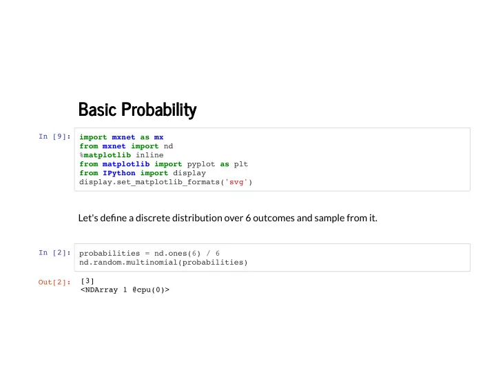
Basic Probability Basic Probability In [9]: import mxnet as mx from mxnet import nd % matplotlib inline from matplotlib import pyplot as plt from IPython import display display.set_matplotlib_formats('svg') Let's de�ne a discrete distribution over 6 outcomes and sample from it. In [2]: probabilities = nd.ones(6) / 6 nd.random.multinomial(probabilities) [3] Out[2]: <NDArray 1 @cpu(0)>

Let's draw from it multiple times. In [3]: print(nd.random.multinomial(probabilities, shape=(10))) print(nd.random.multinomial(probabilities, shape=(5,10))) [3 4 5 3 5 3 5 2 3 3] <NDArray 10 @cpu(0)> [[2 2 1 5 0 5 1 2 2 4] [4 3 2 3 2 5 5 0 2 0] [3 0 2 4 5 4 0 5 5 5] [2 4 4 2 3 4 4 0 4 3] [3 0 3 5 4 3 0 2 2 1]] <NDArray 5x10 @cpu(0)>

Let's see what happens for 1000 samples. In [4]: rolls = nd.random.multinomial(probabilities, shape=(1000)) counts = nd.zeros((6,1000)) totals = nd.zeros(6) for i, roll in enumerate(rolls): totals[int(roll.asscalar())] += 1 counts[:, i] = totals To start, we can inspect the �nal tally at the end of rolls. In [5]: totals / 1000 [0.167 0.168 0.175 0.159 0.158 0.173] Out[5]: <NDArray 6 @cpu(0)>

Let's look at the counts. In [6]: counts [[ 0. 0. 0. ... 165. 166. 167.] Out[6]: [ 1. 1. 1. ... 168. 168. 168.] [ 0. 0. 0. ... 175. 175. 175.] [ 0. 0. 0. ... 159. 159. 159.] [ 0. 1. 2. ... 158. 158. 158.] [ 0. 0. 0. ... 173. 173. 173.]] <NDArray 6x1000 @cpu(0)>

Normalizing by the number of tosses, we get: In [7]: x = nd.arange(1000).reshape((1,1000)) + 1 estimates = counts / x print(estimates[:,0]) print(estimates[:,1]) print(estimates[:,100]) [0. 1. 0. 0. 0. 0.] <NDArray 6 @cpu(0)> [0. 0.5 0. 0. 0.5 0. ] <NDArray 6 @cpu(0)> [0.1980198 0.15841584 0.17821783 0.18811882 0.12871288 0.14851485] <NDArray 6 @cpu(0)>

In [10]: plt.figure(figsize=(8, 6)) for i in range(6): plt.plot(estimates[i, :].asnumpy(), label=("P(die=" + str(i) +")")) plt.axhline(y=0.16666, color='black', linestyle='dashed') plt.legend() plt.show()