AUTOMATED REASONING Otten "Restricting Backtracking in - - PowerPoint PPT Presentation

AUTOMATED REASONING SLIDES 11: ASPECTS OF TABLEAU THEOREM PROVING Controlling Backtracking Universal Literals in Model Elimination

KB-AR - 13 Variants and extensions to Model Elimination In these slides we consider two extensions to Model Elimination; 1) Variation in the search mechanism: The method of removing potentially redundant backtracking (called non-essential back-tracking by the author) has been proposed by Jens Otten "Restricting Backtracking in Connection Calculii" (2010). Although the method is not complete, it has proved to be very effective in practice. A large proportion of problems can be solved with the restriction, and the average saving in search time allows for more complex proofs to be found that would not be found by standard model elimination in a reasonable time. Shown in Slides 11a. 2) Universal Literals: When discussing Re-Use we saw that in first order ME it may be possible to derive universal lemmas of the form ∀z.R(z), which can then be used elsewhere in the tableau. Such universal literals can arise in other ways and we discuss how to exploit

• this. Shown in Slides 11b/c.

3) The OPTIONAL slides 9-11 Appendix 2 also show three Case Studies for your interest: Case Study 1 - KE Tableaux: This variation of tableau uses a single splitting rule; Case Study 2 - Intermediate Lemma refinement (ILE): This is a variant of model elimination; Case Study 3 - Relation between Clausal Tableau and Model Generation (MG) 11ai 11aii

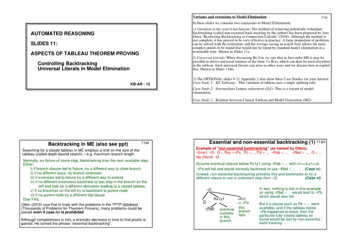
Backtracking in ME (also see ppt)

Searching for a closed tableau in ME employs a limit on the size of the tableau (called depth-bound search) – e.g. maximum branch length. Normally, on failure of some step, backtracking tries the next available step: Either: i) if branch closure led to failure, try a different way to close branch ii) if no different ways, try branch extension iii) if extension led to failure try a different way to extend iv) if no different extensions backtrack to last step in the branch on the left and look for a different derivation leading to a closed tableau v) if no branches on the left try to backtrack to parent node vi) if no parent node try a different top clause Else FAIL Otten (2010) saw that in trials with the problems in the TPTP database (Thousands of Problems for Theorem Provers), many problems could be solved even if case iv) is prohibited. Although completeness is lost, a dramatic decrease in time to find proofs is

• gained. He coined the phrase "essential backtracking".

11aiii Example of "non-essential backtracking" (as named by Otten): Given: ¬G, G ∨ Rxy ∨¬Px, Pc ∨..., Pd ∨..., ¬Rab ∨ ..., ¬Rbd ∨ ..., G ∨ ... top clause ¬G Assume eventual closure below Rx1y1 using ¬Rab ∨ ... with x1==a,y1==b ¬Pa will fail and would normally backtrack to use ¬Rbd ∨ ... (Case iv) Instead, non-essential backtracking prohibits this and backtracks to try a different clause to use in extension step from ¬G (Case vi)

Essential and non-essential backtracking (1)

Rx1y1 G ¬Px1 ⇒ ¬Pa ¬Rab ¬G eventual success in this branch this branch fails In fact, nothing is lost in this example as using ¬Rbd ∨ ... would lead to ¬Pb which would also fail. But if a clause such as Pb ∨ ... were available, and if the tableau below ¬Pb happened to close, then the particular fully closed tableau so found would be lost by non-essential back-tracking

11aiv Example of "essential backtracking" (as named by Otten): Given: ¬G, G ∨ Rxy ∨¬Px, Pc ∨..., ¬Rab ∨ X, ¬Rbd ∨ Y, ¬Rcd , Assume no eventual closure below Rx1y1 using ¬Rab ∨ X then backtrack (essential backtracking) to use ¬Rbd ∨ Y (Case iii) Suppose closure obtained with binding x1==b,y1==d (Case iv) Suppose failure beneath resulting ¬Pb (then normally would backtrack to Rx1y1 Back-tracking to use ¬Rcd is pruned, even though ¬Pc might succeed Otten called this (pruning of) "non-essential" backtracking

Essential and non-essential backtracking (2)

Do not backtrack to try ¬Rcd because it's non-essential back-tracking –case (iv) and is pruned Try to match ¬G with another clause; no clause so fail Lose solution using ¬Rcd Rx1y1 G ¬Px1 ⇒ ¬Pa ¬Rab ¬G failure in this branch X Rx1y1 G ¬Px1 ⇒ ¬Pb ¬Rbd ¬G success in this branch Y failure in this branch by essential back-tracking Case iii 11av Formalising Essential Backtracking and Non-Essential Backtracking: Consider a Model Elimination derivation that is part completed, such that the next leaf node to be extended is L in branch B. Assume also that L could close using any of the literals at N1, N2, ..., Nk in B (above L) and could be extended using any of the matching clauses R1, R2, ..., Rm. Then the method of Essential Back-tracking allows every one of the Ni and the Ri to be tried (in order) to close the tree. This is the normal kind of systematic back-tracking. The method of Non-essential Back-tracking truncates the list of choices as soon as one of them succeeds in closing a sub-tableau beneath L. As a consequence, if any other branch in the tableau to the right of B should fail to close, then there will be no back-tracking to try a different choice at L. In the Example on 11aiv, beneath Rx1y1 the matching clauses are ¬Rab ∨ X, ¬Rbd ∨ Y and ¬Rcd. ¬Rab ∨ X fails and so ¬Rbd ∨ Y is tried. This succeeds and it's assumed Y can be closed, but although the branch below Px1 (now Pb) fails, non-essential backtracking has truncated the choices so ¬Rcd is no longer available to try as an alternative beneath Rx1y1. 11avi Consequences of ignoring non-essential backtracking:

• Loss of completeness (See 11aiv)
• Irrelevant back-tracking is by-passed in a simple way (See 11 aiii)
• Proof search is therefore much faster, allowing harder proofs to be found

Essential and non-essential backtracking (3)

Why does this back-tracking restriction not lose many proofs? There are usually several different ways to make a ME derivation from a set of clauses, each derivation differing in the order in which the clauses are used, and/or the instances used. Disregarding non-essential back-tracking simply searches for

• ne of the other orders, or one of the other derivations.
• Example. Given: ¬G, G ∨ Rxy ∨¬Px, Pa ∨..., G ∨ Pb, ¬Rab ∨ X, ¬Rbd

Assume Closure below X is ok and also Closure below ¬Pb is ok Rx1y1 G ¬Px1 ⇒ ¬Pa ¬Rab ¬G success fails X (1) (1) fails; if Case iv is prohibited then don't find (2); after changing matching clause for ¬G (3) succeeds by Case vi. Check the instances in (3) are the same as those in (2) Rx1y1 G ¬Px1 ⇒ ¬Pb ¬Rbd ¬G (2) Pb G Pb G Rx1y1 ⇒ Rby1 ¬G ¬Rbd ¬Pb G (3) 11bi Example Given: 1. Rx ∨¬Px, 2. Px ∨Q, 3. ¬Ra ∨¬Rb, 4. ¬Q

An Extension to ME Tableaux (see ppt motivation)

(Non-) Standard ME Tableau Resolution Refutation (5 = 2+1): Rx ∨Q (6 = 5+3): ¬Rb ∨Q (7 = 6+5): Q ∨Q ⇒ Q (9 = 8+4): [ ] vs. Q** Px1 ¬Px2 Rx2⇒Rx1⇒Ra ¬Ra x1==a ¬Rb Px3⇒Pb Q ¬Px4 ¬Q ¬Q Rx3 x2==x1 x4==x3 x3==b corresponds to the resolution step ¬Rb ∨Q + Rx3 ∨Q ⇒ Q ∨Q Can merge Q with Q** Merge step corresponds to Q ∨Q ⇒Q Notice that clauses 5 and 6 correspond to the leaf literals of the open branches after each of the first 2 steps of ME. Compare step giving (7) with ME: Instead of standard ME tableau below ¬Rb repeat enclosed part of the tableau below ¬Rb but with new free variables x3 and x4, which will bind to b instead of a.

11bii Example Given: 1. Rx ∨¬Px, 2. Px ∨Q, 3. ¬Ra ∨¬Rb, 4. ¬Q

An Extension to ME Tableaux (motivation)

(Non-) Standard ME Tableau Resolution Refutation (5 = 2+1): Rx ∨Q (6 = 5+3): ¬Rb ∨Q (7 = 6+5): Q ∨Q ⇒ Q (9 = 8+4): [ ] vs. Q** Px1 ¬Px2 Rx2⇒Rx1 ¬Ra x1==a ¬Rb ¬Q x2==x1 The idea will be to retain the ME structure by treating literals such as Rx1, which do not share variables with other open branches, as being universally quantified In this way, Rx1 is effectively written as ∀ ∀ ∀ ∀x. Rx, hence considering it to be used as (Rx11 ∧ ∧ ∧ ∧ Rx12 ∧ ∧ ∧ ∧ ... ∧ ∧ ∧ ∧ Rx1k), setting k big enough to give as many instances as required Features of Universal Variables:

• bindings to x1 cannot affect literals

in other open branches;

• once a free variable becomes

universal it cannot lose this status as long as the convention for bindings

• n closure given on Slide 11cvi is

followed; 11ci

Generalised Closure Rule and Universal Variables (1)

Let T be a partially developed ME tableau and B be an open branch of T. If free variable x1 occurs in some literal in B and and the only occurrences

• f x1 in an open branch are in branch B, then x1 is called a universal

variable in T.

• we'll see that a Universal variable is essentially universally quantified - as

many (different) copies as may be needed are ( implicitly) available

• simulated by not propagating bindings made to a universal variable,

leading to the Generalised Closure Rule (GCR) Closed C[x1] B[x1] No x1 here More Features of Universal Variables 11cii

Generalised Closure Rule and Universal Variables (2)

Closed C[x1] B[x1] No x1 here D[x1] x1 is not universal Closed- no binding to x1 x1 is now universal

• a free variable x1 might not be

universal in T when first introduced into a tableau T, but can become so if x1 eventually occurs in a single open branch; e.g. if branches to left of B[x1] close without binding x1, then x1 in B[x1] is not universal as D[x1] is still open to its

• right. If B[x1] closes without binding x1

then x1 is universal in D[x1].

• if a variable occurs in only one literal

in a clause it will be universal when used in a tableau e.g. y will be universal when using S∨P(x,y)∨Q(x) Let T be a partially developed ME tableau and B be an open branch of T. If free variable x1 occurs in some literal in B and and the only occurrences

• f x1 in an open branch are in branch B, then x1 is called a universal

variable in T. 11ciii Generalised Closure Rule (GCR): The slides 11b and 11c illustrate and explain an extension for ME-tableaux called the generalised closure rule, which exploits the concept of a universal variable. For the simplest case, let C be a clause in which variable u occurs in exactly one literal L. u is called a universal variable. The quantifier for this variable could (implicitly) be distributed across to L. When the clause is developed, one can treat L as if it were ∀u.L, implicitly including in the tableau branch containing L several copies of L, each with a fresh free variable for u. (Any non-universal variable in L would be substituted by exactly one free variable, the same one in all copies.) Since there are always available enough copies for each different binding, an implementation can effectively ignore bindings for u, giving rise to the generalised closure rule. This rule states that in any closure step involving a universal variable u possible bindings to u can be ignored. e.g. if L is P(v,u), and u is universal but v is not, then L is regarded as if it were ∀u.P(v,u) and can be copied in the tableau branch as P(v1,u1), P(v1,u2), etc., for example giving possibility of closure with ¬P(a,b)∨¬P(a,c). If L is part of a clause such as L∨ Q(w), the duplication treats the clause as if it had the more general form of (P(v,u1)∧P(v,u2))∨Q(w). More generally, let T be a partially developed ME tableau and B be an open branch of T. If free variable x1 occurs in some literal L[x1] in B and the only occurrences of x1 in an

• pen branch are in branch B, then x1 is called a universal variable in T and the literal L is

treated as ∀x.L[x].

11civ Rx ∨¬Px, Px ∨Q, ¬Ra ∨¬Rb, ¬Q In Px ∨Q, x is universal. The clause Px1∨Q is used in the tableau as the equivalent ∀ ∀ ∀ ∀x.P(x) ∨ ∨ ∨ ∨Q. At closure (1) use instance P(x2) of ∀x.P(x). Rx2 becomes universal and is treated as equivalent to ∀x.R(x). At closure (2) use instance R(a) of ∀x.R(x). At closure (3) use instance R(b) of ∀x.R(x).

Example Revisited (1)

Q Px1 ⇒∀x.P(x) ¬Px2 Rx2 ⇒∀x.R(x) ¬Ra (2) ¬Rb ¬Q (1) (3) None of the bindings made affects the branch beneath Q, since the universal variables do not appear in it. That branch only needs to be completed once. Implementing Universal Variables: Either tag a universal variable and always use a fresh copy, (so here it is x2 that is bound to the fresh copy of x1 - i.e. "fresh copy" ==x2 - not the other way around) or replace by the universal quantifier (easier when working by hand).

• Exercise (Not easy!):

Consider whether, and how, use of the generalised closure rule could be used in a tableau together with either the (re-use) and/or the (merge) closure rules. 11cv Rx ∨¬Px ∨ Sx, Px ∨Q, ¬Ra ∨¬Rb, ¬Q After closure (1) x2 in Rx2 is not universal (x2 occurs in sibling Sx2) At closure (2) use x2==a At (3) must use a fresh copy of clause Rx ∨¬Px ∨ Sx At (4) bind x3==b At (5) can use an instance of ∀x.P(x)

Example Revisited (2)

Q Px1 ⇒∀x.P(x) ¬Px2 Rx2 ¬Ra (2) ¬Rb ¬Q (1) (3) Sx2 ⇒ Sa Rx3 ¬Px3 ⇒ ¬Pb (4) Sx3 (5) ⇓ Sb 11cvi

An Important Criterion (when implementing GCR) (1)

In making a closure that involves at least

• ne universal variable always introduce a

fresh copy of the universal variable to make the closure. Px1 (∀x.P(x)) ¬Px2 Rx2 (1) Sx2 x1 not in here Example A: In normal ME, to close at (1) either make binding x1==x2, or x2==x1; it doesn't matter which. In GCR it is important to introduce a fresh copy of x1 and to set "fresh copy"==x2. This is achieved in an implementation by tagging x1 as universal and always using a fresh copy. (Otherwise, if x2 and x1 were simply bound to each other, then x1 would in effect be propagated to both Rx2 and Sx2 and x1 would lose its universal status.) 11cvii

An Important Criterion (when implementing GCR) (2)

Example B: when closing at (2), remember to use a fresh copy of implicit ∀x.R(x) and set "fresh copy"==x3; then at (3) it is important to use a fresh copy of implicit ∀x.¬P(x) and set "fresh copy"==x1. Otherwise, x2 and x1 would be bound to each other via x3 and x2 would lose its universal status, which would affect the literal Rx2 as well and could compromise the proof beneath (4). In making a closure that involves at least one universal variable always introduce a fresh copy of the universal variable to make the closure. P(x1) ¬Py2 Rx2 (∀x.R(x)) S(x1) ¬Rx3 ¬Px3 (∀x.¬P(x) (2) y2==x1 x3 not in here (4) (3)

Generalised Closure Rule – Criterion for Maintaining maximal Universality of Variables: Example: Let x be a universal variable in a leaf of branch B of tableau T, say in Q(x), and some step use the clause instance ¬Q(z1)∨ R(z1)∨ S below it. One of the implicit instances of ∀x.Q(x) is Q(x1) and x1 can be bound to z1. In the literal R(z1), z1 will now be universal, since if x was universal then no occurrences of x occurred in T other than in B, and the same applies to the extension of B ending in leaf node R(z1) (branch B', say). In effect, ∀z.R(z) has been derived in B'. To see this, add the negation ¬∀z.R(z) to the tableau and see that the tableau will close if S can close. A variable becomes universal in this way in a Model Elimination tableau if it does not occur in any leaf literals in open branches to its right in the tableau. In this example that is the case, as explained. It is assumed that as construction of a tableau progresses variables are implicitly marked as universal whenever possible, in the manner described in the previous example. That is, a free variable x occurring in leaf literal L in an open branch B is marked as universal if the only

• ccurrence of x in a leaf literal in an open branch is in L. [Observe that (non-universal)
• ccurrences of x could only occur in the branch above L if the occurrence of x in L was
• riginally z (say) and arose because z was bound to x by a clause used in the closure of one of

L's left (closed) siblings. Note x would not be classified universal in L in this case.] In the example on slide 11di: the variable y2 is bound to y1 and hence y1 in R(y1) is not universal. L is originally R(y2), becoming R(y1) , when ¬A(x2,y2) closes with ∀x.A(x,y1), binding y2 to y1. All occurrences of y1 remain non-universal. Exercise: The criterion for choosing closure bindings is: In making a closure involving ≥1 universal variables introduce fresh copies of the universal variable(s) to make the closure. Explain why this assures that any variable declared universal will remain so during subsequent tableau development. 11cviii 11di Normal Form Representation of a Partial Tableau (or Why does the Generalised Closure Rule work?) Consider the standard ME tableau after closure (1) The open branches ≡ ∀y1∀x1[(A(x1,y1) ∧ (P(x1) ∨ R(y1)) ∨ B(y1)] ≡ ∀y1 [(∀x.A(x,y1) ∧ (∀x.P(x) ∨ R(y1)))∨ B(y1)] ≡ ∀y[(∀x.A(x,y) ∧∀x.P(x))∨ (∀x.A(x,y) ∧R(y))∨ B(y)] That is, maximally distribute ∀. Given: (1) ¬P(a)∨ ¬A(b,z) (2) ¬R(c)∨ ¬A(c,c) (3) A(x,y)∨B(y) (4) ¬A(x,y)∨P(x)∨R(y) A(x1,y1) B(y1) ¬ A(x2,y2) x2==x1 y2==y1 (1) P(x2) ⇒ P(x1) R(y2) ⇒ R(y1) Using universal variables treats universal literals as quantified literals as in the above expression. You can see that x1 in A(x1,y1) and in P(x1) are universal, and that y1 is not universal. See next slide for rest of tableau. 11dii Continued from Slide 11di After closure (1) (above the wavy line), and making universal variables explicit, the

• pen branches ≡ ∀y[(∀x.A(x,y) ∧∀x.P(x))∨ (∀x.A(x,y) ∧R(y))∨ B(y)] (*)

(1) ¬P(a)∨∀z.¬A(b,z) (2) ¬R(c)∨¬A(c,c) (3) ∀x.A(x,y)∨B(y) (4) ¬A(x,y)∨P(x)∨R(y) Variables z and x in givens (1) and (3) are universal, as indicated. After closure (1) can ``forget’’ the bindings to universal variable x in ∀x.A(x,y1); also x2 in P(x2) becomes universal. At (2) instances A(x3,y1) and A(b,z3) are unified (x3, z3 being the fresh copies

• f x and z) leaving y1 unbound.

At (3) y1 is bound to c and at (4) ¬A(c,c) unifies with A(x4,c), x4 the fresh copy of x in ∀x.A(x,y1) => ∀x.A(x,c). The last open branch contains B(c). Notice B(c) is derivable from (*),(1), (2). ∀x.A(x,y1) B(y1)⇒ B(c) ¬ A(x2,y2) y2==y1 (1) P(x2) (∀x.P(x)) R(y2) ⇒R(y1) ¬P(a) ∀z.¬A(b,z) ¬R(c) y1==c ¬A(c,c) (2) (3) (4) Soundness of the Generalised Closure Rule: Justification that the generalised closure rule is sound can be made by appealing to the expression represented by the open part of a partial tableau, distributing quantifiers maximally across literals containing universal variables. The ``open part'' of any tableau (i.e. the set of branches not yet closed) typically represents a universally quantified formula in dnf; i.e. a disjunction of (possibly quantified) conjunctions

• f literals. This was illustrated on slide 11di. Suppose a new clause is added to the leftmost
• pen branch. Assume that non-universal variables in the added clause are always renamed

as fresh free variables. When a new clause is added in an extension step there are two options for forming the binding in the closing unifier for a variable x: either x is universal and a fresh copy of x becomes bound, or x is not-universal and is bound in the normal way. Thus e.g. when matching ∀x.A(x,y1) with ∀z.¬A(u1,z), the universal fresh copy x2 of x in A(x2,y1) is bound to u1, and the fresh copy z2 of z in ¬A(u1,z2) is bound to y1 (ie "fresh copy–x"==u1 and "fresh copy_z"==y1). The open part of the extended tableau can be recomputed and universal quantifiers distributed to maximise occurrences of universal variables. Assuming the criterion on slide 11cvi is adhered to, it is not hard to show that universal variables remain so. Given the dnf representation of the open part of a partial tableau (call it dnf(T) ), it is then easy to show that if T" is derived from T then dnf(T) |= dnf(T"). 11diii

11ei

• Prolog-like - use stacks for implementation (but: need to detect ancestors,

and use the occurs check)

• Prolog technology: compilation, structure sharing, stack maintenance
• Easy to obtain variations
• Easy to implement in Prolog
• Easy to extend to modal logics (and others)
• Consider a problem Data |– P → Q. Clausal form of ¬(P → Q) is P and ¬Q.

May want to work forwards from P and "backwards " from ¬Q. In ME must choose one of them as top clause.

• May be beneficial to resolve some clauses initially if they only resolve with
• ne or two others. i.e. a non-linear beginning.
• Left-Right depth first generation of search space may not be the smallest.
• Quite often the search space contains several variations of the same

refutation, in which the clauses are used in different orders. (It is this property that was exploited in non-essential backtracking removal.)

Summary of Advantages of ME-style tableaux Disadvantages

11fi

Summary of Slides 11

• 1. The Model Elimination (ME) tableau method can be extended and modified in

various ways.

• 2. The introduction of universal variables and the generalised closure rule that

results leads, in many cases, to reduced tableaux. Universal variables are treated in the tableau as being universally quantified, instead of as free variables, so multiple instances are allowed. This leads to the generalised closure rule, which is implemented by not propagating bindings to universal variables (in effect such bindings are ignored).

• 3. ME tableau are complete. However, some completeness can be sacrificed

through pruning back-tracking of the "non-essential" kind. It turns out that in many problems involving unsatisfiable data, while some completeness is lost, in that not all refutations can be found, it is still possible to find at least one refutation.

• 4. ME style tableau have advantages, especially in that they are easily

implementable in Prolog, which is good for testing new ideas. All the Prolog technology is available to build good systems. The method extends to other logics, e.g. modal logic.

• 5. ME style tableau have disadvantages, mainly related to their being linear.

S ST TA AR RT T

• f

f O OP PT TI IO ON NA AL L M MA AT TE ER RI IA AL L ( (S SL LI ID DE ES S 1 11 1) )

Motivating GCR in more detail (see also slides A2e in Appendix A2 for slides 9-11)

11gi Example Given: 1. Rx ∨¬Px, 2. Px ∨Q, 3. ¬Ra ∨¬Rb, 4. ¬Q

An Extension to Basic ME Tableaux (1)

As in Slide 11bi but showing standard ME tableau. Notice that clauses 5 and 6 correspond to the leaf literals of the open branches after each of the first 2 steps of ME. Compare step 3 (giving (7)) with ME: Q Px1⇒Pa ¬Px2 x2==x1 Rx2=>Rx1 ⇒Ra ¬Ra x1==a ¬Rb Rb ¬Pb Pb Q ¬Q ¬Q Cannot unify Rb with Rx2 here as x2 has been bound to a. Standard ME Tableau Resolution Refutation (5 = 2+1): Rx ∨Q (6 = 5+3): ¬Rb ∨Q (7 = 6+5): Q ∨Q ⇒ Q (9 = 8+4): [ ] vs.

11gii Example Given: 1. Rx ∨¬Px, 2. Px ∨Q, 3. ¬Ra ∨¬Rb, 4. ¬Q

An Extension to Basic ME Tableaux (2)

Instead of standard ME tableau below ¬Rb try repeating 1st 2 steps below ¬Rb (blue part of the tableau) but with new free variables x3 and x4, which will become bound to b instead of a. In some cases can avoid actual

• duplication. e.g. here would

close at the leaf ¬Rb (implicitly matching a second copy of Rx1). Results in the generalised closure rule. Notice that x1 does not occur in any open branch to the right of the branch ending at ¬Rb. In the fresh instance of the enclosed tableau the branch below Q can be closed by a merge with Q**, so simulating the resolution proof. Q** Px1 ¬Px2 Rx2⇒Rx1⇒Ra ¬Ra x1==a ¬Rb Px3⇒Pb Q ¬Px4 ¬Q ¬Q Rx3 x2==x1 x4==x3 x3==b corresponds to the resolution step ¬Rb ∨Q + Rx3 ∨Q ⇒ Q ∨Q Can merge Q with Q** Merge step corresponds to Q ∨Q ⇒Q 11giii Given: 1. Rx ∨ ¬Px, 2. Px ∨ Qx, 3. ¬Ra ∨ ¬Rb, 4. ¬Qa

An Extension to Basic ME Tableaux (3)

In some cases cannot avoid actual duplication. Notice that x1 now occurs in two branches, including the open branch to the right of the branch ending at Rx1, in Qx1. In the fresh instance of the enclosed tableau the 2nd branch below ¬Rb becomes Qb, which doesn't merge any more with Qa. It is incorrect to avoid the duplication as the branch below Qb would be lost leading to the wrong result, since this branch fails. Qx1⇒Qa** Px1 ¬Px2 Rx2⇒Rx1⇒Ra ¬Ra x1==a ¬Rb Px3⇒Pb Qx3⇒Qb ¬Px4 ¬Qa Rx3 x2==x1 x4==x3 x3==b corresponds to the resolution step ¬Rb ∨Qa + Rx3 ∨Qx3 ⇒ Qb ∨Qa