AUTOMATED REASONING lectures. They're included for interest and are - - PowerPoint PPT Presentation

AUTOMATED REASONING OPTIONAL SLIDES Appendix A2 (Tableau Extras) CASE STUDY 1 - KE tableau CASE STUDY 2 - Intermediate Lemma Extension Model Generation (propositional prover) RELATIONS between RESOLUTION and TABLEAU Completeness of Resolution via tableaux A very useful notation (chain notation) Relation of ME with linear resolution The UNIFY - AT - END tableau development Brief look at Parallel Model Elimination

KB-AR - 13 A2ai These slides cover various topics about the tableau method, for which there isn't time in the

• lectures. They're included for interest and are completely OPTIONAL! They discuss:

i) Case Study 1: The KE tableau prover; this alternative tableau method has just one splitting rule - either P or ¬P - and has some theoretical interest, in that it has better complexity than standard tableaux. It has not been investigated as much as ME tableau, especially at first order

• level. It has similarities with the DP method and could be viewed as a first order version of the

Davis Putnam Procedure; ii) Case Study 2: A variant of ME is the Intermediate Lemma Extension. This has some similarities with Neg-HR, and is a tableau version; iii) There is a useful alternative to Davis Putnam for propositional logic called Model

• Generation. It is related to tableau, which allows to give a simple prof of its correctness;

iv) an alternative proof of the completeness of resolution using tableau; v) a discussion of the relation between linear resolution and ME tableaux. Linear resolution is a refinement in which each new resolvent is formed by resolving the previous resolvent with either a given clause or another resolvent. The first step resolves two given clauses. This is related to the extension step of Model elimination; vi) The constrained development of model elimination tableaux allows for a concise notation to represent an ME tableau as a list of literals, which in turn allows a whole search space to be depicted in the plane (Chain Notation); vii) Also included are some slides on Unify-at-end and parallel development of tableaux. Appendix A2 – Tableau Extras A2bi Case Study 1: The KE Tableau Method A first order implementation exists by Tomas Chrien (2013) (MSc project) (There are still many extensions and improvements - a good project!) The KE tableau method is more recent than other techniques, having been introduced only in the last 15 years or so. (See "The Taming of the Cut", D'Agostino and Mondadori, and also Endriss: A Time Efficient KE Based Theorem prover.) In the first order case there has been very little work

• n practical theorem provers, so the example here is illustrative only. The KE rules can be viewed

either as generalisations of the Davis Putnam steps or as variations of ordinary tableau rules, trying to retain much of the ME method, but for arbitrary sentences. There is just one splitting rule, but it is not restricted to atoms. The non-splitting rules are similar to the DP steps which prune atoms, and for clauses they are exactly the same. KE is more efficient than standard tableau, unless Re- use (see Slide 10ciii) is included in tableaux development. In that case (for clausal form) KE- tableaux can be simulated by ordinary ME-tableau +Re-use. In the first order example on Slide A2bv it is appropriate to draw the universal quantifiers into a prefix, but more generally, this may not be so. Similar benefits to those provided by universal variables might be obtained if universal quantifiers are distributed as much as possible, but this remains to be investigated, as does the possibility of eliminating non-essential backtracking. In the example on A2bv the first step uses the (¬∧) rule, together with the free variable ∀ elimination rule to derive ¬pr(n) from (4) and div(x2,x2). The next step anticipates the use of the(→) rule and sets this up by a PB application using ¬(div(g(x1),x1) ...). In the second branch of the PB the(→) rule is used several times, in combination with free variables. The KE method is quite human oriented in the ground case. But it is quite hard in the first order case because of the various ways that the (∀) rule can be combined with other rules. It tends to give rise to much less branching than ME tableau. A2bii

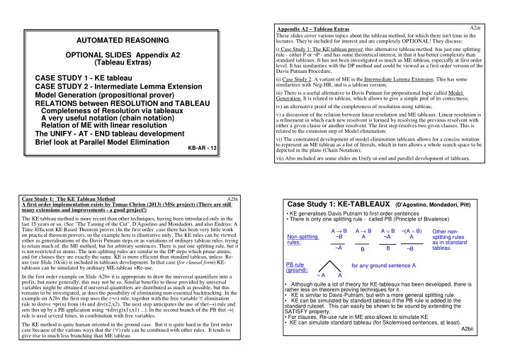
Case Study 1: KE-TABLEAUX (D'Agostino, Mondadori, Pitt)

• KE generalises Davis Putnam to first order sentences
• There is only one splitting rule - called PB (Principle of Bivalence)
• Although quite a lot of theory for KE-tableaux has been developed, there is

rather less on theorem proving techniques for it.

• KE is similar to Davis-Putnam, but with a more general splitting rule.
• KE can be simulated by standard tableau if the PB rule is added to the

standard ruleset. This can easily be shown to be sound by extending the SATISFY property.

• For clauses, Re-use rule in ME also allows to simulate KE
• KE can simulate standard tableau (for Skolemised sentences, at least).

Other non- splitting rules as in standard tableau A → B ¬B ¬A A ∨ B ¬A B ¬(A ∧ B) A ¬B A → B A B Non-splitting rules: ¬ A A for any ground sentence A PB rule (ground):

A2biii Given data:

• 1. a ∧ w → p 2. i ∨ a 3. ¬ w →m, 4. ¬ p 5. e → ¬ i∧ ¬ m 6. e

¬p e ¬ i ∧ ¬ m (5, →rule) ¬i (∧rule) a (2, ∨rule) ¬ (a ∧ w) (¬∧rule) ¬ w (∧rule) ¬m (3, →rule) m

• []

a ∧ w (PB) p (1, →rule)

• []

KE seems to be good for propositional tableaux. The amount of branching is generally lower than for standard tableaux

Example of KE

The PB rule is often used to introduce the second premise for the non- splitting rules. e.g. see the use of PB on a ∧ w above. PB rule (non-ground): for new free variables x in sentence A ¬ A[x] A[x]

• The ∃-rule and ∀-rule are the same as for ordinary free-variable tableau;
• One method to deal with quantifiers is to draw them into a prefix and use free

variable tableaux rules. These are often combined with one of the two-premise

• rules. See example on next slide.
• Little investigation of heuristic techniques for first order KE have been made to

date, so far as I'm aware. (Tomas Chrien's MSc project 2013 made a start.)

• Soundness and Completeness have been shown for the ground case.
• The KE-approach has proved useful for modal logics as well.
• Clausal KE is quite similar to Davis Putnam, effectively providing a first order

version of it.

First Order KE rules

A2biv A is any first order formula or literal eg ∃x(Px ∨ Qx), R(x1,y1), etc. Given: (1) ¬(div(g(x),x) ∧ less(1,g(x)) ∧ less(g(x),x) ) → pr(x) (2) div(u,w) ∧ div(w,z) → div(u,z) (3) less(1,x)∧less(x,n)→div(f(x),x)∧pr(f(x)) (4) ¬(pr(y)∧div(y,n)) (5) div(x,x) (6) less(1,n) div(x2,x2) (∀) (5) ¬ pr(n) (∀, ¬∧) (4) ¬(div(g(x1),x1)∧less(1,g(x1)) ∧ less(g(x1),x1)) pr(x1) (1, ∀→)

• x1==n

div(g(x1),x1) ∧ less(1,g(x1)) ∧ less(g(x1),x1) ⇒div(g(n),n) ∧ less(1,g(n)) ∧ less(g(n),n) div(g(n),n), less(1,g(n)) ∧ less(g(n),n) (∧) div(f(g(n)), g(n)) ∧ pr(f(g(n))) (3, ∀→) div(f(g(n)), g(n)), pr(f(g(n))) (∧) A2bv (u,w,x,y,z are universally quantified) div(u1,w1)∧div(w1,z1) div(u1,z1) (2, ∀→) ¬ pr(u1) (4, ∀¬ ∧) z1==n

• u1==f(g(n))

¬(div(u1,w1)∧div(w1,z1)) ⇒ ¬(div(f(g(n)),w1)∧div(w1,n)) ¬div(g(n), n) (¬ ∧) w1==g(n)

• First Order KE example

(PB) (PB) Soundness and Completeness for Ground KE (Outline) The soundness of ground KE is simple to show; it is sufficient to show the property SATISFY for the non-splitting rules and the PB rule. SATISFY is obviously true for an application of the PB rule (say for the sentence A), since the model of the branch before the rule must assign either T or F to A; if it assigns T then the branch below A will still be satisfiable and if it assigns F then the branch below ¬A will still be satisfiable. For the other rules, consider the exemplar A, ¬(A∧B) ==> ¬B. If a model M satisfies a branch containing the formulas A, ¬(A∧B), then M will clearly satisfy ¬B, the conclusion of the rule. It is also quite easy to show correctness (soundness and completeness) in a manner similar to that used for DP on Slides 1. This is not a coincidence, since KE is very similar to DP, especially if all sentences are clauses. We define the α-rules to be those rules which are α-rules of ordinary tableau, and the β-rules to be the remaining non-splitting rules (e.g. A and ¬(A∧B) ==> ¬B). The minor sentence in a non-branching KE rule application of the β-kind is the smaller sentence (e.g. A in the above example rule). There are then basically 5 cases: a contradiction between a sentence and its negation, no sentences left to develop in a branch, an application of an α-rule, a sentence S used as the minor sentence in a β-rule application, and a PB application. However, the proof similar to that used for DP requires the KE derivation to make all applications of a β-rule using the chosen minor sentence at once. Since this is not necessarily the normal or best way to make a KE derivation we'll give a different proof for completeness for ground KE. See A2bvii. A2bvi

Completeness for Ground KE (Continued) Each sentence that occurs as a (sub)formula in the given data is a potential candidate for a β-rule application and is called a given sub-formula. (Note that atoms occurring in a given sentence are counted as given sub-formulas.) An open branch of a ground KE tableau is called fully developed if every given sub- formula in the branch, or its negation, occurs at a node in the branch and no further rule applications are possible. Clearly, there is no need to use PB for any given sub-formula that already appears in a branch. Let S be a given set of sentences and suppose a KE tableau is found with a fully developed open branch B. From this branch a model for S can be found in a similar way to that described for standard tableau and shown to satisfy the sentences in the branch. The proof for satisfiability is by contradiction from the asumption that some smallest sentence in B is false. For example, suppose such a smallest false sentence was of the form X∨Y. Then both X is false and Y is false. Since B is fully developed either X or ¬X is in B. If it is X then this contradicts the assumption that X∨Y is a smallest false

• sentence. If it is ¬X then the (∨) rule would have derived Y, again a contradiction. The
• ther cases are similar and full details are left as an exercise.

Therefore, if S is an unsatisfiable set of sentences, then no fully developed open branch can exist and the KE tableau must close. For the first order case the method is essentially similar. A reasonable way to develop a KE tableau is thus to use the α-rules and β-rules as much as possible, only using PB to introduce the minor sentence for a β-rule application. The amount of splitting is then kept to a minimum. A2bvii A2ci Given ¬Paa, ¬Pf(a)a ∨¬Paf(a), Pf(a)a ∨¬Q ∨Paa, Paf(a) ∨ Paa, Q ∨R, ¬R In a similar way can derive Paf(a) by using Paf(a) ∨Paa instead of Pf(a)a ∨¬Q ∨Paa (Called Intermediate Lemmas) Intermediate Lemma Extension:

• 1. Select a positive literal from each

non-Horn clause as the conclusion literal of that clause. Other positive literals are called lemma literals.

• 2. Proceed as in Prolog - begin from

an all-negative clause, match with "conclusion" literals and ignore other positive literals that arise unless they match the immediate parent.

Case Study 2: Generalising Prolog to arbitrary clauses

Step 1: choose (and underline) conclusion literals Step 2: derive lemmas. Can derive Pf(a)a ∨ R from above tableau: add ¬(Pf(a)a ∨ R) and derive a closed tableau. If positive literals Pf(a)a and R are ignored then tree is complete ¬Paa Paa Pf(a)a

|– Pf(a)a ∨ R

¬Q Q R Ground clause example Step 3: Find lemmas Pf(a)a ∨ R and Paf(a). Step 4: Use these lemmas to form lemma R Step 2/3: Find a refutation. A2cii

• 3. Either - find a refutation - no lemma

literals left as leaves; Or - derive a lemma - only lemma literals left as leaves; form a lemma from the disjunction of all leaf literals.

• 4. Deal with the lemma as in 1, then can try

an alternative path in 2, using new lemma. ¬Pf(a)a ¬Paf(a) Pf(a)a Paf(a) R Form lemma R. ¬R R Can piece together the various tableaux used to obtain lemmas to form a closed tableau - it will not be a regular nor a ME tableau. In the example, in the final refutation, replace use of lemma R by tableau used to derive R, then replace use of other lemmas by tableaux used to derive them. (See A2ciii.)

Intermediate Lemma Extension (contd.):

Given: ¬G, G ∨¬Pxy ∨¬Pyx, Pf(u)u ∨Pua, Pvf(v) ∨Pva A2ciii ¬G G ¬Px1y1 ¬Py1x1 Px1a Pf(x1)x1 Paa Pf(a)a ⇒ ¬Px1a ⇒ ¬Pax1 x1==a ⇒ Pf(a)a Tableau 1 finding lemmas. Pf(a)a∨ Pf(a)a factors to Pf(a)a If lemma is L∨M (open branches ending in L and M) then can close tableau by placing ¬(L∨M) ≡ ≡ ≡ ≡ ¬L∧¬M as an initial sentence in the tableau. So L∨M really is a lemma. e.g. Pf(a)a is implied by tableau 1 and Paf(a) is implied by tableau 2. ¬G G ¬Px3y3 ¬Py3x3⇒ ¬Pax3 Px3a Px3f(x3) Paa Paf(a) x3==a y3==a ⇒ Paf(a) Paf(a) ∨ Paf(a) factors to Paf(a) Tableau 2 finding lemmas. General clause example

A2civ Example of a more general lemma: open branches ending in P(x) and Q(y,x) lead to a lemma ∀xy [P(x) ∨ Q(y,x)]. Adding ¬ ∀xy [P(x) ∨ Q(y, x)] to the initial set of sentences, which Skolemises to the two facts ¬P(a), ¬Q(b, a) for new a and b, will enable the tableau to close. The method seems to be fairly efficient: In effect, many sub-tableau of small depth are joined together to form a large

• tableau. (When a lemma is

used the tableau which derived it could be used instead.) Because the individual search spaces are small the total search is reduced. Given: ¬G, G ∨ ¬Pxy ∨ ¬Pyx, Pf(u)u ∨ Pua, Pvf(v) ∨ Pva, Lemmas: Pf(a)a, Paf(a) (found as on 11diii) Use lemma 2 (Paf(a)) ¬G G ¬Px2y2 ¬Py2x2⇒ ¬Paf(a) Pf(a)a x2==f(a) y2==a Use lemma 1 (Pf(a)a) beneath ¬Px2y2. Tableau 3 using lemmas Paf(a) A2cv Intermediate Lemma Extension (1): The Intermediate lemma extension on slides A2c is a hyper-resolution (or Prolog)-like extension for tableaux. (Don't confuse with other ME-extensions called hyper-tableaux - see TABLEAUX conferences.) In any clause with at least one positive literal, exactly one positive literal is marked as the conclusion literal. Other positive literals (if any) are called lemma literals. (If a clause has exactly one positive literal it is the conclusion.) Each clause with no positive literals is called a goal clause and can be used as a top clause. For uniformity, a new literal "G" can be appended to each goal clause (then all given clauses will have at least one positive literal). The top clause is then a new clause, ¬G. A ME-tableau is constructed from the top clause, in which the lemma literals are initially ignored – branches in which they occur as leaf literals are not pursued. (An extension allows the lemma literals to close a branch (if possible) by matching some earlier negative literal in the branch. This reduces the length of the eventual lemma.) If a tableau closes and there are no ignored lemma literals then this indicates that a refutation has been found. Otherwise, if a tableau closes and there are ignored lemma literals, the lemma literals are put into a new clause (i.e. the new clause is the disjunction of the lemma leaf literals), which is added to the data and called an intermediate lemma. This clause will have only positive literals, and one is chosen as the conclusion literal. Only intermediate lemmas that are not subsumed need be added. Clauses that are subsumed by the new intermediate lemma can also be removed. In case an intermediate lemma is retained, a new attempt at a refutation from ¬G (or a top clause) can be made using all given clauses and all non-subsumed intermediate lemmas. Factoring can be incorporated in two different ways. Either: (i) clauses can be (safe-factored) before being accepted (either as a given clause or as an intermediate lemma), or (ii), a positive literal that would otherwise be ignored may be matched with its parent (if possible). I prefer the first method, since it allows for all safe-factors to be found regardless of which positive literal might be selected as a conclusion literal. The second method is more dependent on the selection

• f conclusion literals to detect safe-factors. However, it is simpler to implement.

A2cvi Intermediate lemma Extension (2): The process of forming lemmas and refutations needs to be controlled in some way, analogous to setting depth limits in the standard ME procedure. The simplest is the following: All possible ways of closing a tableau descended from ¬G are formed and all intermediate lemmas formed, both upto some initial fixed depth. Then the process is repeated, but making use of the new clauses as well. If no further tableaux can be formed at the given depth and no refutation has been found then the process is repeated but to a greater depth. Unfortunately, the depth may need to be increased even though new intermediate lemmas can be found at the current depth. e.g. initial clauses include ¬Q, P(a), Q∨¬P(x)∨P(f(x)). Together, if Q is the conclusion literal in the third clause, these allow for the lemmas P(f(a)), P(f(f(a)), etc. to be formed, all at depth 2, even though none of these lemmas may be the ones required for a

• refutation. To overcome this problem make a lemma contribute more than 1 to the depth-count

when it is used in a refutation. e.g. make a lemma count exactly 1+number of lemmas used in its

• derivation. This is consistent with giving an initial clause a count of 1, since it uses no lemmas in

its derivation. Hence, at a given depth there is a maximum number of lemmas that can be used and a finite number of possible refutations that could be made. Once a refutation has been found, a complete tableau can be constructed from the various tableaux used to form the lemmas. Beginning with the last used lemma, the use of each lemma is replaced by the tableau that derived it. All its leaves will match in the same way that the lemma

• did. This substitution of tableaux can be repeated until all lemmas have been replaced.

In the tableau on A2ci/ii, first the tableau for R is used beneath ¬R. This tableau uses the clauses Pf(a)a ∨R and Paf(a), which are also lemmas. They are replaced by the tableaux which derived them, the leaf literals that formed the lemmas now matching where those of Pf(a)a ∨R or Paf(a)

• did. See diagram on A2cvii.

A2cvii Soundness and Completeness of the Intermediate lemma Extension: Next we show that the method of the Intermediate Lemma Extension is both sound and complete (at the ground level). The ground level tableau can then be lifted to give completeness and soundness at the general level in a similar way to that used for free variable tableau on slides 9. To show soundness, note that each generated lemma is associated with a sub-tableau. These various sub-tableaux can be used in place of the corresponding lemma, as described on A2cvi. Each closure that was possible using the conclusion literal of the lemma is still possible using the tableau. For the example on A2ci/ii the final closed tableau is shown above. Intermediate Lemma Extension: Reconstructing a closed tableau from lemmas Replace tableaux deriving lemmas Pf(a)a ∨R and Paf(a) ¬R ¬Pf(a)a ¬Paf(a) Pf(a)a Paf(a) R (1) (2) (3) ¬Paa Paa Pf(a)a ¬Q Q R ¬R ¬Pf(a)a ¬Paf(a) ¬ Paa Paa Paf(a) (1) (2) (3) In closed tableau from 11dii with top clause ¬R and closure with lemma R replace R with the tableau on 11dii that derived it

Completeness of the Intermediate Lemma Extension: The proof is by induction on the number of lemma literals in the given clauses. Let S be a minimally unsatisfiable set of clauses with a total of k lemma literals. (i.e. if any clause is removed from S then S would become satisfiable.) If k=0 then the clauses are Horn clauses and since S is unsatisfiable there will be at least one all-negative clause in the set-of-support. Then there is a standard ME tableau starting from this all-negative top clause that will close (by completeness of ME). It is not hard to show the structure of the closed tableau is of the right form (and simulates a Prolog derivation from S). If k>0, suppose as induction hypothesis (IH) that, for 0≤m<k lemma literals, there is always a set of sub-tableaux formed using the method, which can be pasted together to give a closed and soundly formed tableau. Let C be a clause with a lemma literal L and let C'=C-{L}. Form S'=S-{C}+{C'} and S''=S-{C}+{L}. Each may be made minimally unsatisfiable such that, for the case of S', C' is needed to show unsatisfiability, and in the case of S'' {L} is

• needed. (Show this by using the assumption that S is minimally unsatisfiable). Since in both S'

and S'' the number of lemma literals <k, by IH there is constructable a well-formed Intermediate Lemma tableau from an all-negative clause for S' and for S''. Now take the constructed tableau for S' and put back L into C', forming C again. The tableau for S’ was closed but will now give rise to the lemma L: in the derivation of the tableau for S’, use of C (where before C' was used) will include using L, multiple occurrences all being factored to give the lemma L. In the well-formed tableau for S'', this tableau deriving lemma L can now be used wherever originally the clause L was used. A2cviii A2cix For the example on A2ci/ii the choices made for L are: R from Q ∨R, Pf(a)a from Paa ∨Pf(a)a ∨¬Q and Paf(a) from Paa ∨ Paf(a); lemma atoms are non-conclusion atoms. There are 3. (Conclusion atoms are underlined.) Assume C1 is Paa ∨ Paf(a), giving C1'= Paa. S1'={Q ∨R, ¬R, Paa ∨Pf(a)a ∨¬Q, Paa, ¬Paa, ¬Pf(a)a ∨¬Paf(a)}, which reduces to minimally unsatisfiable {Paa, ¬Paa}, and S1''={Q ∨R, ¬R, Paa ∨Pf(a)a ∨¬Q, Paf(a), ¬Paa, ¬Pf(a)a ∨¬Paf(a)}. In S1'' choose as C2 the clause Paa ∨Pf(a)a ∨¬Q, and use the IH to form tableaux from S2'={Q ∨R, ¬R, Paa ∨¬Q, Paf(a), ¬Paa, ¬Pf(a)a ∨¬Paf(a)} and S2''={Q ∨R, ¬R, Pf(a)a, Paf(a), ¬Paa, ¬Pf(a)a ∨¬Paf(a)}. For S2' choose C3=Q ∨R and S3'={Q, ¬R,Paa ∨¬Q, Paf(a), ¬Paa, ¬Pf(a)a ∨¬Paf(a)} and S3''={R, ¬R}. The tableaux for S3'', S2'', S1' are fairly obvious. Tableau (i) below is for S3'. After re-inserting L3=R into S3' can use it in closure for S3'', as shown in (ii). Two more constructions are needed to complete the full tableau according to the proof. These are left as an exercise for you. Paa ¬Q (i) Q ¬Paa ¬Paa Paa (ii) ¬Q Q R ¬R An Assessment of the Intermediate Lemma Extension: In 2010 MSc student Rosa Gutierrez Escudero implemented various refinements for the ILE and performed a thorough set of benchmarking tests using the TPTP (Thousands of problems for theorem provers) Database. It turned out that the method generally performs no better than Model Elimination as implemented in the best standard version of LeanCop (with Re-Use but no backtracking restrictions). The method was tested on problems including equality, and using various ways to reason with equality. (However, recently she has made the code more efficient, so there may be an update.) In one variant the lemma literals were not restricted to be positive atoms. Instead, it was allowed for a uniform translation to be applied to literals in the initial clauses. That is, certain literals could be transformed into their complements. (This is similar to the transformation described for generalising hyper-resolution.) For some problems this proved to be a good

• improvement. Whereas the normal ILE method restricts lemma literals to be atoms,

transforming (say) all P literals into their complements will not affect unsatisfiability, but may affect the syntactic structure of the clauses and lead to a simpler derivation. The ILE method might be expected to perform well – in order to construct a derivation it searches many small search spaces for the lemmas. However, many lemmas are derived more than once and therefore subsumed and hence redundant; this appears to be one reason that ILE is not as good as might be expected. e.g. suppose the lemma A ∨ B is found at depth 3. Then when additional lemmas are sought using any newly found lemmas, A ∨ B will be found for a second time. Subsumption is important though, as if A in A ∨ B is marked as conclusion, the next lemma may well be B, subsuming the previous lemma. Secondly, non-essential backtracking was less helpful – the restrictions on forming a tableau are quite strict in ILE, so alternative derivations were often not allowed. A2cx

A2di

• Example. Given: ¬B ∨ ¬M, M ∨ ¬L, M ∨ L ∨ ¬B, B ∨ R, ¬R

A: Form a tableau such that no literal occurs twice in a branch, and every internal node is matched by a leaf node. B: Each clause with leaf nodes only can be resolved with the literal just above. e.g. clause labelled (1). ¬B ¬M B R M ¬L ¬R B R M L ¬B ¬R (1) C: The tableau is adjusted by removing the resolved literals from the two clauses

• involved. e.g. ¬B from

(1) and B from B∨R. The remaining literals still match above and the tableau still closes. e.g. Simulates formation of resolvent M∨L∨R. NOTE: M∨L∨¬B can be removed from beneath ¬B as M does not match below. Then M∨¬L can be removed similarly. ¬B ¬M M ¬L M L ¬B B R ¬R

Completeness of Resolution using Tableaux

A2dii ¬B ¬M B M M (4) ¬L L (5) ¬M M M 1: M∨L∨¬ B + B∨R ⇒M∨L∨R 2: ¬R + B∨R ⇒ B 3: ¬R + M∨L∨R ⇒ M∨L 4: B + ¬B∨ ¬M ⇒¬M 5: M∨L + M∨ ¬ L ⇒ M∨M ⇒M 6: ¬M + M ⇒[] After each step, it is still the case that no literal occurs twice in a branch and all internal nodes are matched by a leaf node. Also, the tableau is properly closed still, but using (some of) the original clauses as well as any new resolvent. It may be necessary to factor. e.g. Before step (6) must factor M∨M to M. ¬B ¬M B M ¬L R ¬R M L (3) R ¬R (2) A2diii Another Proof of Completeness for Resolution: The slides A2d give a constructive proof that refutation by ground resolution (and factoring) is complete, but this time based on the completeness of tableau systems. The idea is to build a closed (ground) tableau from the given clauses and then to transform it in small steps, each step corresponding to a resolution step. In Stage A a closed ground regular tableau is formed with the properties that (i) every non-leaf node is complemented by a leaf node and (ii) no branch contains a literal more than once. (Note that a ME tableau would satisfy (i) and (ii) initially, but so do some other tableau as well.) In order to achieve this, if n is a non-leaf node in clause C that is not complemented, then C is removed from the tableau and the sub-tableau beneath n can descend directly from its parent since no closures use n. (See example.) If n is a node

• ccurring twice in a branch, then the clause containing the occurrence at greater depth

can be removed and the sub-tableau beneath n can descend directly from its parent as any closures can use the remaining occurrence. In Stage B clauses are removed from the tableau starting from all-leaf clauses. The parent

• f such a clause C must match with at least one literal in C, given that property (i) of

Stage A is true. Thus C can be resolved (possibly with factoring of the matching literal) with the clause D containing its parent. The resolvent replaces D in the tableau. The properties (i) and (ii) of Stage A are maintained and the tableau still closes. If there were an exception, it would contradict that the property held before the resolution step. Exercise: show these 3 things. After none or more resolvents have been formed, a tree occurs of the form X(¬X) at a node m, with one or more occurrences of ¬X(X) at child nodes of m. The corresponding resolution step (including factoring) results in the empty clause. Since every step removes at least 1 closure, the process will terminate.

A2ei Relation between ME tableau and Linear resolution refinements (1) ME-tableaux are closely related to the linear refinement of resolution. This refinement is

• utlined below. It was introduced long before free-variable ME-tableaux, as were the various

restrictions of the refinement. However, there is one particular restriction, called SL- resolution, which corresponds exactly to free-variable ME-tableau. When the generalised closure rule is included, then more general linear resolution proofs can be simulated by

• tableaux. The relationship between the two systems is detailed further in the chapter notes on

clausal tableaux on my website, if you're interested. Strategy of Linear resolution First select an initial clause called top in the set of support of set of clauses S: The set of support of S = {C |C ∈S and S-{C} is satisfiable}; i.e. each C in the set of support is necessary to derive [ ]. Next resolve C with an input clause from S (possibly a second copy of top). Then, at each subsequent step resolve the latest resolvent with either an input clause, or a previous resolvent (called ancestor resolution). e.g. If the refutation is R0 , R1 , R2 , ...., [ ], where R0 is the top clause, then R2 is formed by resolving R1 with an input clause, or with R0, or with R1. Linear resolution appears to be quite natural as it generalises top-down/goal-directed

• reasoning. The search space is a tree, each branch being one possible linear derivation, so

efficient search methods and Prolog technology can be employed. The top clause and subsequent resolvents in the example shown on the right in A2bv are: Px ∨Q, Rx ∨Q, ¬Rb ∨Q, Q∨Q (i.e. Q), [ ].The ancestor resolution step is between ¬Rb ∨Q and Rx ∨Q, deriving Q∨Q, which factors to Q. A2eii Relation between ME tableau and Linear resolution refinements (2) Next we explain how a ME-tableau relates to a linear resolution derivation. The idea is that at each ME-step the disjunction of the leaf literals in open branches is the latest resolvent of the corresponding linear refutation. In the example on A2bv, after the first closure the leaf literals

• f the open branches are Rx and Q, which are exactly the literals in the second resolvent in the

derivation, as given in A2bi. Similarly, after the second closure the leaf literals are ¬Rb and Q, exactly the third clause in the derivation. The various tableau steps correspond as follows: i) Extension corresponds to resolution of an input clause with the latest resolvent, ie one that has been extended in the branch before, choosing to resolve on a literal most recently introduced into the resolvent. ii) Closure corresponds to resolution of the latest resolvent with an ancestor resolvent, but in a quite restricted way. If the previous resolvent used was R = L ∨ C, where L was the literal resolved upon in R before, then R can only be used again by resolving on L. Moreover, the same "instance" of R must be used. That means that both copies of R must use the same instantiation, i.e. it is R used twice, not R and a copy of R. This is sufficient to ensure that the 2 occurrences of clause C in the resolvent that arise from the two steps using R will factor. In fact, as long as this latter property holds, the other restriction can be relaxed; this would correspond to using the generalised closure rule. In a normal ME tableau, the restriction on closure is automatically ensured by the structure of the tableau, since only one instance of each literal occurrence is allowed. On A2ev, notice that in order to use Rx a second time with substitution b, it is necessary to use a second occurrence, which brings with it a second occurrence of Q. The same effect can be obtained by allowing a second instance of Rx (namely when x==b), as in the generalised closure rule of ME. As an example, A2ev shows the linear refutation corresponding to the LH tableau of 11bi. A2eiii Model Elimination Tableau Simulation of Linear Resolution Consider the tableau shown on A2eiv and the corresponding linear resolution derivation, which is also shown. The top clause of the linear derivation is Fx1∨Hx1, which is the first clause in the ME tableau. The first two steps resolve with input clauses and the resolvents of each step correspond to the leaf literals of the open branches of the tableau. Notice that the third step, which resolves with Fx1 for a second time and which derives Hb ∨Hb, is an ancestor matching step in the tableau and that there is only one instance of Fx1, which is the

• ne enforced by the unifier of this step. The two occurrences of Hb appear just once in the
• tableau. In the resolution proof the resolution is between the clause ¬Fb ∨Hx1 and a copy of

the ancestor Fx1∨Hx1, say Fx3∨Hx3, which yield Hb ∨Hx1. This factors to Hb and corresponds with the tableau version. The restricted linear resolution strategy, which simulates ME, only allows resolution with the ancestor instance Fx1∨Hx1, not a fresh copy of Fx ∨Hx. It also restricts to using Fx1, the literal prevously resolved upon. If that instance were to be used later in the derivation, it is only the instance Fb ∨Hb that may be used. The unrestricted liner resolution strategy will also allow ¬Fx2 to resolve with a fresh copy of the ancestor Fx ∨Hx. In the tableau, the ancestor matching step (corresponding to using the copy) is made explicitly because Fx1 from Fx1∨Hx1 is not part of the "history" leading to ¬Fx2. The generalised closure rule corresponds to using the copy to resolve with the current resolvent R, as long as the copy of the remaining literals safely factors with the literals in R. In general linear resolution the step of ancestor resolution is even more flexible - any literal in the ancestor can be used, not just the literal that was used the first time the ancestor was involved in a resolution step. More on this is in the `Chapter' notes if you're interested. Fx1∨Hx1 ¬Fx ∨Gx} {Gx1∨Hx ¬Gx ∨ ¬Fb} ¬Fb ∨Hx1 Hb ∨Hb Hb ⇓ ¬Hb ∨ ¬Fx ¬Fx2 Fx ∨Hx Hx2 ¬Ha x1==b (x2==a) [ ] A2eiv Comparison of Linear resolution and ME for the clauses: ¬Ha , ¬Gx ∨ ¬Fb , ¬Fx ∨ ¬Hb , Gx ∨ ¬Fx, Fx ∨ Hx ¬F(x2) x2==x1 Fx1 Hx1 ⇒ Hb G(x2) ⇒Gx1 ¬Hb ¬ Fx2 ¬Gx1 Fx2 Hx2 ¬Fb x1==b ¬Ha x2==a See A2eiii for commentary on these derivations

A2ev Generalised closure rule of ME can simulate Linear Resolution Rx ∨ ¬Px, Px ∨Q, ¬Ra ∨ ¬Rb, ¬Q A ME tableau can be seen as simulating a special kind of linear resolution strategy. In the derivation on the right the two copies of Q derived from the same parent literal will factor. This will always be the case in the tableau if variables in the branch closing by the generalised closure rule do not occur in any remaining leaf literals. A linear resolution strategy. Q Px ¬Px Rx ¬Ra x=a ¬Rb Px Q ¬Px ¬Q ¬Q =>Ra Rx Px ∨Q ¬Px ∨Rx Rx ∨Q ¬Ra ∨¬Rb Q ∨Q ¬Q ¬Rb ∨Q [ ] A2fi Chain Notation for ME Tableaux: For interest, slide A2fii shows a convenient representation for ME-tableaux, called the chain notation, which is possible because such tableaux are developed from left to right. This notation enables a complete search space to be represented in 2 dimensions. A ME-tableau is maintained as a chain of literals. There are two types of entry, boxed and un- boxed literals. The top clause forms the first chain with the leftmost literal the next to be selected and all literals unboxed. A chain may (i) be extended by a new clause, (ii) be extended by ancestor matching or (iii) be truncated, corresponding, respectively, to tableau extension, ancestor closure or moving to the next branch to develop. (i) results in the matched literal becoming boxed and literals in the (added) matching clause (not including the complementary literal) being appended to the left of the chain. (ii) results in the leftmost literal being boxed if it unifies with a boxed literal to its right. (iii) removes leftmost boxed literals. A chain represents the remaining open branches of the ME tableau formed so far, which can be re-constructed from the chain. Each unboxed literal is a leaf literal L of the tableau. Its ancestors, forming the rest of the branch, are all the boxed literals to its right (the first boxed literal to the right being the parent of L). Alternatively, all literals to the left of a boxed literal are its decendants. The example on A2fii illustrates. Regular tableaux can be enforced by not allowing a step that would result in an unboxed literal being duplicated by another boxed literal to its right. Also, if an unboxed literal is duplicated by an unboxed literal to its right, then the leftmost literal can be boxed, corresponding to the "merge" operation. A2fii ¬B∨ ¬M, M∨ ¬L, M∨L∨ ¬B, B∨R, ¬R top clause ¬B¬M extension R ¬B ¬M extension R ¬B ¬M truncation ¬M extension L¬B ¬M extension M L ¬B ¬M ancestor matching M L ¬B ¬M truncation ¬B ¬M extension R ¬B ¬M extension R ¬B ¬M truncation [] ¬B B R ¬R ¬M M L ¬B ¬L M B R ¬R Regularity: If a literal occurs in a chain twice, the leftmost unboxed, the right

• ccurrence boxed, the leftmost indicates

a duplication.

CHAIN NOTATION - A handy shorthand

Merging: If a literal

• ccurs in a chain twice,

both times unboxed, the leftmost can be merged with the right copy.

Model Generation Procedure (MG): Another procedure appropriate for propositional clauses is model generation (MG), which is a special case of the tableau method. MG is easy for humans to use as it is more restricted than DP, which you saw in Slides 1. Slides A2 give some examples of MG and a correctness proof. The MG procedure attempts to build partial models. It constructs a tree in which each branch tries to maintain a partial model of the initial sentences (but in a different way to DP). The tree built by the MG procedure for an initial set of clauses S consists of nodes each labelled by an atom. There are 2 kinds of branches, called open and closed. The atoms in each open branch B give a model of the set of clauses processed in B; when all of S have been processed in an open branch B then the branch is called completed and the nodes in B give rise to a (partial) model of S. A closed branch B is also called completed and indicates that the atoms in B cannot be extended to be a model of S (i.e. they make some clause in S false). Let closed branches be labelled by false and completed open branches be labelled by true. Then the given clauses S have no model if the disjunction of all labels in a tree in which all branches are completed is false. There is a model if the disjunction is true, as at least one branch must then have been completed and open. Proof of the correctness of the MG procedure uses notions of tableaux. A2gi A2gii

Model Generation Example (tree form) (Rules on A2giii)

Given clauses S: LK, ¬L¬K, ¬LM, ¬MK, MR (ie L∨K etc.) Checks: no tautologies and no subsumed clauses, (initial checks) at least one negative literal (step 1) MG(S,{ }) (ie the branch is empty) Choose LK (step 2) MG([¬L¬K, ¬LM, ¬MK, MR],{L}) Choose ¬LM (step 2) MG([¬L¬K, ¬MK],{L,M}) Choose ¬MK (step 2) MG([¬L¬K],{L,M,K}) choose ¬L¬K return False (step 3) MG([¬L¬K, ¬LM, MR],{K}) Choose MR (step 2) MG([¬L¬K],{K,M}) return True (step 4) Model={K,M,¬L} (Must make L False as K already True) MG(([¬L¬K, ¬LM],{K,R}) return True (step 4) Model={K,R,¬L} Return (False or True or True) =True- hence there's a model L M K K M R A2giii

Model Generation Procedure

MG is initially called with S=given clauses and B= [ ]. procedure MG(S,B): boolean %S are clauses still to make true and B is the branch (model) so far

• 1. If no clause in S contains a negative literal then return true.

(B is a partial model of the initial clauses)

• 2. If S contains a clause C with ≥1 positive literals such that for all negative

literals ¬L in C (if any), L occurs in B, then return disjunction of MG(S(Ai),B+Ai) , for each positive literal Ai in C, where S(Ai) = S - {X|X in S and X made true by assignments in B+Ai}

• 3. If S contains a clause C with only negative literals such that for all literals

¬L in C, L occurs in B, then return false. (B makes C false)

• 4. If none of 1, 2 or 3 occurs then return true.

(Every remaining clause has ≥1 literal ¬L, where L is not in B) MG(S,B) halts with true if S+B has a model and returns a partial model that includes B (ie makes atoms in B true) and which can be extended to a complete model for S+B (see Notes on the procedure). MG(S,B) halts with false if S +B has no models. procedure MG(S,B): boolean

• 1. If no clause in S contains a negative literal return true.

Note1: B satisfies all clauses so far removed from the original argument S. B can be made into a model of the remaining clauses by assigning true to any atoms not yet assigned, since they either occur positively in S, or do not occur at all. (Covers the case when S is empty. )

• 2. If C = E ∨ D (where all literals Ai in E are positive and ¬Lj in D are negative) is in

S and for all ¬Lj in D, Lj is in B, then return disjunction of MG(S(Ai),B+Ai) , for each Ai in E Note2: The branches of the form B+Ai extending B are the only ways to make C

• true. Can remove any clauses in S also made true by B+Ai (for the Ai branch)
• 3. If C in S has only negative literals and for all literals ¬Li in C, Li is in B, then

return false. Note3: B cannot be extended to make C true as it already makes C false.

• 4. If none of 1, 2 or 3 occurs then return true.

Note4: Every remaining clause in S has ≥1 unassigned negative literal ¬L. Assign false to all such L to make the remaining clauses true. Can assign either true or false to any remaining atoms in the language not yet assigned. A2giv Some Notes about MG These notes are to give you some intuition as to why the MG method works. You can assume there are no tautologies or subsumed clauses at the start and that all identical literals have been merged.

Example: {LK, ¬L¬K, ¬LM, ¬MK, MR} (a slightly different tree than that shown on A2gii) (Step 2) Choose MR (could also have chosen LK instead as on Slide 2bii). Return MG([LK,¬L¬K, ¬MK], {M}) or MG([LK,¬L¬K, ¬LM, ¬MK], {R}); i.e. start a tree with two branches. Consider the first disjunct and (Step 2), clause ¬MK. Return MG([¬L¬K], {M,K}). ie still to make ¬L⁄¬K true (Step 4) return true - assign false to L. Check that {M,K,¬L} is a (partial) model for the initial clauses. If the second disjunct had been chosen, then apply (Step 2) and clause L⁄K and return MG([¬L¬K, ¬LM, ¬MK], {R,L}) or MG([¬L¬K, ¬LM], {R,K}); i.e. extend the second branch of the tree by two branches. The first disjunct will eventually return false (show this yourself) and the second will return the model {R,K,¬L}. Check that {R,K,¬L} is a (partial) model for the initial clauses. A2gv Exercises: 1)Use MG on the "three little girls" problem. 2) Consider how a purity rule might be included into MG 3) Can you suggest any efficiency short cuts for MG? The data (1) C(d) ∨ C(e) ∨ C(f) One of the threee girls was the culprit (2) C(x) → H(x) { C(d) → H(d), C(e) → H(e), C(f) → H(f) } To convert into propositional form (3) ¬(C(d) ^ C(e)) (4) ¬(C(d) ^ C(f)) (5) ¬(C(f) ^ C(e)) Only one of the three girls was the culprit (6) C(d) ∨ H(d) ∨ ¬C(e) (Dolly's statement negated) (7) C(e) ∨ C(f) ∨ ¬(C(e) → (C(d) ∨ H(d))) (Ellen's negated) (8) C(f) ∨ ¬H(d) ∨ ¬((H(d) ^ C(d)) →C(e)) (Frances's negated)

"The three little girls" problem again!

A2gvi This time we’ll try to find a model and return True (and we hope the model will make C(f) true). We convert to clauses and can remove any tautologies or subsumed clauses at the start. Also merge identical literals (1) C(d) ∨ C(e) ∨ C(f) (2a) ¬C(d) ∨ H(d) (2b) ¬C(e) ∨ H(e) (2c) ¬C(f) ∨ H(f) (3) ¬ C(d) ∨ ¬C(e) (4) ¬ C(d) ∨ ¬C(f) (5) ¬ C(e) ∨ ¬C(f) (6) C(d) ∨ H(d) ∨ ¬C(e) (7a) C(e) ∨ C(f) ∨ C(e) (7b) C(e) ∨ C(f) ∨ ¬C(d) (7c) C(e) ∨ C(f) ∨ ¬ H(d) (8a) C(f) ∨ ¬H(d) ∨ H(d) (8b) C(f) ∨ ¬H(d) ∨ C(d) (8c) C(f) ∨ ¬H(d) ∨ ¬C(e)

Solution to "The three little girls" by MG

A2gvii Merge literals in (7a) to obtain C(e) ∨ C(f) and remove (8a) (tautology); (7a) subsumes (7b), (7c), (1); call MG( [2a, 2b, 2c, 3, 4, 5, 6, 7a, 8b, 8c], [] ); Apply (Step 2) on 7a (C(e) ∨ C(f)); evaluate MG([2a, 2b, 2c, 3, 4, 5, 6, 8b,8c], [C(e)] ) (i) or MG([2a,2b,2c,3,4,5,6 ], [C(f)] ) (ii); In (i): apply (Step 2) to 2b and call MG([2a,2c,3,4, 5, 6,8b, 8c], [H(e), C(e)] ); Apply (Step 2) to 6 and evaluate MG([2a,2c,3,4, 5,8c], [C(d), H(e), C(e)] ) or MG([2c,3,4,5,8b, 8c], [H(d),H(e), C(e)] ); Both eventually return false. In (ii): apply (Step 2) to (2c) and call MG([2a, 2b, 3, 4, 5, 6 ], [H(f), C(f)] ); Apply (Step 4) to return true; get the partial model [H(f), C(f), ¬C(d), ¬C(e)]. H(e) and H(d) can be either true or false.

A2gviii

• Similar to the tableau method MG looks for models in each branch

Model Generation (MG) as a Tableau refinement

Example ¬p e ¬e ∨ ¬c ¬a ∨ ¬w ∨ p w ∨ m i ∨ a ¬e ∨ ¬m

• Top clause is always positive ....
• Can extend a branch by clause

C as long as negative literals in C (if any) are complemented in the branch

• All literals in the MG tree (solid

lines) are positive

• Leaf literals, in the tableau,

(dotted lines) are negative literals

• Differences are mainly cosmetic

e w m ¬e ¬m i a ¬e ¬i ¬a ¬w p ¬p A2gix Can we perhaps use the soundness and completeness properties of tableau to show similar properties for MG? Yes, we Can!

Correctness of MG using correctness of Tableaux (1)

Soundness is the easiest If a MG tree for clauses S returns False, then S |= ⊥ If there is a closed tree, it must be because all branches end by using a negative clause, where all its literals are complemented. The implicit tableau would also be closed, and so we use Tableau Soundness to conclude S |= ⊥. e w m ¬e ¬m i a ¬e ¬i ¬a ¬w p ¬p Completeness uses finiteness of MG tree For each open branch B of a MG tree We know that: All clauses with no negative literals are used All unused clauses have negative literals if B were to be extended by any clause with negative literals not yet used in B, there is one extended branch of B which remains open, since all such clauses have one negative literal not matched in B The open branch is saturated and will yield a model A2gx

Correctness of MG using correctness of Tableaux (2)

Example: Remove i ∨ a Open branch (in tableau version of MG) is {e, w, ¬i, ¬a, ¬p} Note - dotted lines are not part of MG tree which ends at w e w m ¬e ¬m ¬e ¬i ¬a ¬w p ¬p If (ground) MG tree is developed left -> right And current open branch includes atoms in an

• pen branch on its right (still to develop)

Then can abandon current open branch See diagram: If branch containing C (and atoms in X) has no model, nor will branch containing {A, B, C} and atoms in X have a model If branch containing C and X does have a model no need to search branch {A,B,C} and X A2gxi

Short cut for MG

Question: Can MG method be generalised to first order clauses? Consider case when signature has no function symbols Either: use analogy with free variable tableau Or: implicitly maintain ground instances of each clause A C C Atoms X B

A2hi How else could the free variable method be systematic? The ME approach is "unify as you go" What about "unify at the end"? How could tableau development be controlled? Possibilities for controlling Unify-at-the-end:

• Restrict total no. of clause instances over all branches / over each branch,
• r number of instances of each clause over all branches / over each branch.
• Likely to get many literals in a branch that cannot possibly unify; the

branches of which they are a part can be pruned. e.g.

• If only one occurrence of Hx in a branch then no need for two instances of

a clause containing ¬H(y), as they would have to be the same.

• If no copies of Hx in a branch then no use for ¬Hy.

Good/bad points of Unify-at-the-end:

• If not many quantifiers "unify at end" may be better.
• May only be one binding for a particular branch. Selecting it can restrict

unifiers in other branches.

• May be able to close branches without unifying. No backtracking (over

those branches).

• May have many unifiers in a branch; all have to be tried.

Comparison between Unify-at-the-end and Unify-as-you-go in ME tableaux An example of this approach is shown on Slide A2 div A2hii Constructing Free Variable Tableaux When constructing a free variable tableau, you may do it in one of two ways, which could be called "unify-as-you-go", or "unify-at-the-end". Slides 9-11 used the unify-as-you-go method and the alternative approach to closure is shown on Slides A2hi/iv: instead of closing each branch "as you go" and propagating the bindings across the whole tableau, it is noted when a branch can close and what the corresponding binding is, but no propagation takes place. The tableau on Slide A2hiii is constructed using "unify-at-the-end". In the construction, if a branch can be closed by unifying two complementary literals, then it is marked as possibly

• closed. All possible unifiers that may lead to closure can be recorded as a label of the branch.

When every branch has such a potential closure, a single unifier must be constructed using one unifier from the label of each branch in the tableau. For the example on A2diii it results in the combined unifier (ie unify the individual unifiers) {x2==w1==g(n), x1==y1==x3==z1==n, u1==f(g(n)), y2==f(g(n))}. If it is not possible to construct a single unifier, then a different set

• f closures must be found (which may involve further extending the tableau) and another

combined unifier sought. This is in contrast to the "unify-as-you-go" kind of construction, illustrated on Slide 9civ, where whenever a closure is made that requires a binding to be made to one or more free variables, the substitution is applied to all occurrences in the tableau of those newly bound variables. This guarantees consistency of the bindings as the tableau is constructed. Only one binding may be made to any free variable. The unify-as-you-go approach is useful for most applications, especially those using data structures, when it may be necessary for a piece of data to be used many times. If it is known (or quite possible that) each sub-sentence of each sentence is to be used only once or a very few times, the unify-at-the-end approach can be a reasonable one. (1) div(x,x), (2) less(1,n), (3) div(u,w) ∧ div(w,z) → div(u,z) (4) ¬(div(g(x),x) ∧ less(1,g(x)) ∧ less(g(x),x) ) → pr(x) (5) less(1,x)∧less(x,n)→div(f(x),x)∧pr(f(x)) Show ∃ ∃ ∃ ∃y (pr(y)∧ ∧ ∧ ∧div(y,n)) A2hiii ¬∃y (pr(y)∧div(y,n)) ¬(pr(y1) ∧div(y1,n)) div(g(x1),x1) ∧ less(1,g(x1)) ∧ less(g(x1),x1) pr(x1) div(f(x2), x2) pr(f(x2)) ¬ (pr(y2)) ∧div(y2,n)) div(u1,z1) ¬ less(1,x2) ¬ less(x2,n) x2==g(x1) x2==g(x1) x1==n (or x2==1 is possible) ¬ div(u1,w1) ¬div(w1,z1) u1==f(x2) w1==x2 z1==x1 w1=g(x1) ¬ pr(y2) ¬ div(y2,n) y2==f(x2) ¬ pr(y1) ¬ div(y1,n) y1==x1 y1==n x3==n div(x3,x3) y2==u1, z1==n Gives: { x2==w1==g(n), x1==y1==x3==z1==n, u1==y2==f(g(n))} Free variable rules Unify at the end A2hiv E.g. Given: Fxa ∨Fg(x)x , Fxa ∨Fxg(x), ¬ Fxa ∨ ¬ Fxz ∨ ¬ Fzx Fx1a Fg(x1)x1 Fx2a Fx2g(x2) Fx3a Fx3g(x3) ¬Fx4a ¬Fx4z1 ¬Fz1x4 ¬Fx5a ¬Fx5z2 ¬Fz2x5 ¬Fx6a ¬Fx6z3 ¬Fz3x6 ¬Fx7a ¬Fx7z4 ¬Fz4x7 Assume at most one instance of each clause will be used in each branch. A successful unification is x4, z1, x1 all bound to a ; i.e. didn't need Fx2a ∨Fx2g(x2) in LH branch - it can be removed - so only need

• ne of the copies of

¬Fxa ∨ ¬Fxz ∨ ¬Fzx x6 bound to x3 and z3 and x3 bound to a; x7 bound to g(a), z4 bound to a.

• Sections of the tableau (indicated by

dotted lines) can be developed in parallel.

• If the tableau is ME style then

possibilities for re-use can be anticipated: eg if S occurs in closure below branch (ii) it can be closed in the same way as the closure below S in branch (i). Anticipate this by adding ¬S to branch (ii). A2hv

Parallel ME : Propositional case

• Each branch of a clausal tableau

can be distributed to a separate thread, or process. This is called and-parallelism as every branch must close for a refutation.

• This is different from or-

parallelism in which each process is instead given a branch of the search space. eg in the tree on the left, if KLM (ie K∨L∨M) matched with more than one clause (as it does here: KLM matches with given clauses ¬KST and ¬K¬S), then there would be two branches of the search space. Process1 is given the search space using ¬KST and process2 the search space using ¬K¬S. If process2 finished before process1 then process1 can be terminated. K L M ¬K S T ¬S ¬K ¬S ¬K ¬K ¬L (ii) (i)

Parallel ME: First Order case

A2hvi

• To cope with potentially infinite tableau in the and-parallel development,

each section is developed to a fixed depth. Failure to find a proof causes the depth to be increased for a second attempt.

• Shared (ie non-universal) variables pose a problem:

e.g. Given: ¬Pxy ∨ ¬Pyx, Pf(u)u ∨ Pua, {Pvf(v) ∨ Pva Pf(u1)u1 Pu1a

• Values of u1 must be reconciled

between two processes.

• Pu1a can close with u1==a. It

can also close with u1==f(a). Q: Are there any more values?

• Within a finite depth the number
• f values will be finite.
• Pf(u1)u1 can also close

(eventually) with u1 ==a.

• Each solution is passed up to

the parent process to be reconciled.

• Only bindings mentioned in

ancestor nodes are retained. ¬Px1y1 u1==x1 y1==a ¬Py1x1 u1==y1 x1==a Reconcile: obtain u1==x1==y1==a; Retain u1==a.

• If u1 were

universal, then can use a technique similar to the generalised closure rule. A2hvii Parallel Clausal Tableau Development: Slides A2hv/vii illustrate some possibilities for and-parallel execution within a clausal tableau. Each branch, called a section on A2hv, can be given to a separate

• processor. It's possible to anticipate some possible cases for re-use as shown on the

slide. The first order case is more complex as bindings must be preserved across branches for the shared (ie non-universal) free variables. One method is for each branch below a node n to be evaluated independently, finding as many bindings as possible for the variables occurring in the literal at n (to some max. depth to guarantee termination). The bindings are then reconciled (i.e. combined) at the node n with those from other sibling branches of n (i.e. only bindings which belong to the solution set of every sibling branch are retained, possibly further instantiated). Finally, only bindings to variables occurring in an ancestor of n need be kept for further propagation. E.g. let ground P occur at n's parent, where n matches with P and let n's siblings be Q(x1) and R(x1). Although x1 must be reconciled with some binding, the particular binding is not relevant to the parent of n, unless x1 occurs elsewhere in the tableau. As this is not the case, the empty binding would be retained to pass back up the

• tableau. However, notice that the following circumstance could occur: x1 is bound

in another branch to some non-universal variable z in some ancestor of n, say x1==z, and also to x1==a, then the reconciled binding z==a is relevant, since z

• ccurs in an ancestor of n. If all reconciliations fail, then no bindings are retained.

A2hvii

Summary of Optional Appendix 2

• 1. The KE prover is an alternative to ME with one splitting rule only. KE is

computationally more efficient than standard tableaux.

• 2. The Intermediate Lemma Extension imposes restrictions to reduce the search space,

but this is offset by requirement for more subsumption tests. It is related to hyper- resolution.

• 3. The completeness of resolution can be shown using tableaux. No doubt, by

controlling the style of tableau formed - e.g. ordering use of clauses in any branch – specific sorts of resolution proofs can be derived.

• 4. ME tableau are related to linear resolution. The correspondence imposes restrictions
• n the linear resolution, which is partially relaxed if the generalised closure rule is used.
• 5. A useful chain notation exists to represent tableau as a list of boxed and unboxed

literals.

• 6. The Model Generation (MG) method for testing satisfiability of propositional clauses

is good for humans, but less well investigated than DP in optimised implementations. MG returns True (and a partial model) for given clauses S if there is one. It returns False if there are no models of S. The returned model (if any) can be extended to all atoms by assigning T or F to unasigned atoms.

• 7. Different unification regimes can be employed in ME tableau, such as ``unify-as-you-

go'', or ''unify-at-the-end''.

• 8. With care ME tableaux can be evaluated in parallel.