[PPT] - Artificial Neural Networks and Deep Learning Christian Borgelt This PowerPoint Presentation

SLIDE 1

Artificial Neural Networks and Deep Learning

Christian Borgelt

Dept. of Mathematics / Dept. of Computer Sciences

Paris Lodron University of Salzburg Hellbrunner Straße 34, 5020 Salzburg, Austria christian.borgelt@sbg.ac.at christian@borgelt.net http://www.borgelt.net/

Christian Borgelt Artificial Neural Networks and Deep Learning 1

Textbooks

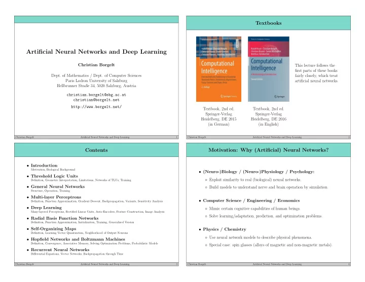
Textbook, 2nd ed. Springer-Verlag Heidelberg, DE 2015 (in German) Textbook, 2nd ed. Springer-Verlag Heidelberg, DE 2016 (in English) This lecture follows the first parts of these books fairly closely, which treat artificial neural networks.

Christian Borgelt Artificial Neural Networks and Deep Learning 2

Motivation: Why (Artificial) Neural Networks?

(Neuro-)Biology / (Neuro-)Physiology / Psychology:
Exploit similarity to real (biological) neural networks.
Build models to understand nerve and brain operation by simulation.
Computer Science / Engineering / Economics
Mimic certain cognitive capabilities of human beings.
Solve learning/adaptation, prediction, and optimization problems.
Physics / Chemistry
Use neural network models to describe physical phenomena.
Special case: spin glasses (alloys of magnetic and non-magnetic metals).

Christian Borgelt Artificial Neural Networks and Deep Learning 4

SLIDE 2

Motivation: Why Neural Networks in AI?

Physical-Symbol System Hypothesis [Newell and Simon 1976] A physical-symbol system has the necessary and sufficient means for general intelligent action. Neural networks process simple signals, not symbols. So why study neural networks in Artificial Intelligence?

Symbol-based representations work well for inference tasks,

but are fairly bad for perception tasks.

Symbol-based expert systems tend to get slower with growing knowledge,

human experts tend to get faster.

Neural networks allow for highly parallel information processing.
There are several successful applications in industry and finance.

Christian Borgelt Artificial Neural Networks and Deep Learning 5

Biological Background

Diagram of a typical myelinated vertebrate motoneuron (source: Wikipedia, Ruiz-Villarreal 2007), showing the main parts involved in its signaling activity like the dendrites, the axon, and the synapses.

Christian Borgelt Artificial Neural Networks and Deep Learning 6

Biological Background

Structure of a prototypical biological neuron (simplified)

nucleus axon myelin sheath cell body (soma) terminal button synapse dendrites

Christian Borgelt Artificial Neural Networks and Deep Learning 7

Biological Background

(Very) simplified description of neural information processing

Axon terminal releases chemicals, called neurotransmitters.
These act on the membrane of the receptor dendrite to change its polarization.

(The inside is usually 70mV more negative than the outside.)

Decrease in potential difference: excitatory synapse

Increase in potential difference: inhibitory synapse

If there is enough net excitatory input, the axon is depolarized.
The resulting action potential travels along the axon.

(Speed depends on the degree to which the axon is covered with myelin.)

When the action potential reaches the terminal buttons,

it triggers the release of neurotransmitters.

Christian Borgelt Artificial Neural Networks and Deep Learning 8

SLIDE 3

Recording the Electrical Impulses (Spikes)

pictures not available in online version

Christian Borgelt Artificial Neural Networks and Deep Learning 9

Signal Filtering and Spike Sorting

picture not available in online version An actual recording of the electrical poten- tial also contains the so-called local field potential (LFP), which is dominated by the electrical current flowing from all nearby dendritic synaptic activity within a volume

f tissue. The LFP is removed in a prepro-

cessing step (high-pass filtering, ∼300Hz). picture not available in online version Spikes are detected in the filtered signal with a simple threshold approach. Aligning all detected spikes allows us to distinguishing multiple neurons based on the shape of their

spikes. This process is called spike sorting.

Christian Borgelt Artificial Neural Networks and Deep Learning 10

(Personal) Computers versus the Human Brain

Personal Computer Human Brain processing units 1 CPU, 2–10 cores 1010 transistors 1–2 graphics cards/GPUs, 103 cores/shaders 1010 transistors 1011 neurons storage capacity 1010 bytes main memory (RAM) 1011 neurons 1012 bytes external memory 1014 synapses processing speed 10−9 seconds > 10−3 seconds 109 operations per second < 1000 per second bandwidth 1012 bits/second 1014 bits/second neural updates 106 per second 1014 per second

Christian Borgelt Artificial Neural Networks and Deep Learning 11

(Personal) Computers versus the Human Brain

The processing/switching time of a neuron is relatively large (> 10−3 seconds),

but updates are computed in parallel.

A serial simulation on a computer takes several hundred clock cycles per update.

Advantages of Neural Networks:

High processing speed due to massive parallelism.
Fault Tolerance:

Remain functional even if (larger) parts of a network get damaged.

“Graceful Degradation”:

gradual degradation of performance if an increasing number of neurons fail.

Well suited for inductive learning

(learning from examples, generalization from instances). It appears to be reasonable to try to mimic or to recreate these advantages by constructing artificial neural networks.

Christian Borgelt Artificial Neural Networks and Deep Learning 12

SLIDE 4

Threshold Logic Units

Christian Borgelt Artificial Neural Networks and Deep Learning 13

Threshold Logic Units

A Threshold Logic Unit (TLU) is a processing unit for numbers with n inputs x1, . . . , xn and one output y. The unit has a threshold θ and each input xi is associated with a weight wi. A threshold logic unit computes the function y =

      

1, if

n

i=1

wixi ≥ θ, 0, otherwise.

θ x1 xn y w1 wn

TLUs mimic the thresholding behavior of biological neurons in a (very) simple fashion.

Christian Borgelt Artificial Neural Networks and Deep Learning 14

Threshold Logic Units: Examples

Threshold logic unit for the conjunction x1 ∧ x2.

4

x1 x2 y

3 2

x1 x2 3x1 + 2x2 y 1 3 1 2 1 1 5 1 Threshold logic unit for the implication x2 → x1.

−1

x1 x2 y

2 −2

x1 x2 2x1 − 2x2 y 1 1 2 1 1 −2 1 1 1

Christian Borgelt Artificial Neural Networks and Deep Learning 15

Threshold Logic Units: Examples

Threshold logic unit for (x1 ∧ x2) ∨ (x1 ∧ x3) ∨ (x2 ∧ x3).

1

x1 x2 x3 y

2 −2 2

x1 x2 x3

i wixi

y 1 2 1 1 −2 1 1 1 2 1 1 1 4 1 1 1 1 1 1 2 1 Rough Intuition:

Positive weights are analogous to excitatory synapses.
Negative weights are analogous to inhibitory synapses.

Christian Borgelt Artificial Neural Networks and Deep Learning 16

SLIDE 5

Threshold Logic Units: Geometric Interpretation

Review of line representations Straight lines are usually represented in one of the following forms: Explicit Form: g ≡ x2 = bx1 + c Implicit Form: g ≡ a1x1 + a2x2 + d = 0 Point-Direction Form: g ≡

x =

p + k r Normal Form: g ≡ ( x − p)⊤ n = 0 with the parameters: b : slope of the line c : section of the x2 axis (intercept)

p :

vector of a point of the line (base vector)

r :

direction vector of the line

n :

normal vector of the line

Christian Borgelt Artificial Neural Networks and Deep Learning 17

Threshold Logic Units: Geometric Interpretation

A straight line and its defining parameters:

x1 x2 g O ϕ c

p
r
n = (a1, a2)
q =

p⊤ n | n|

n

| n|

d = − p⊤ n b = r2

r1

Christian Borgelt Artificial Neural Networks and Deep Learning 18

Threshold Logic Units: Geometric Interpretation

How to determine the side on which a point y lies:

n = (a1, a2)

x1 x2 g O ϕ

y
z
q =

p⊤ n | n|

n

| n|

z =

y⊤ n | n|

n

| n|

Christian Borgelt Artificial Neural Networks and Deep Learning 19

Threshold Logic Units: Geometric Interpretation

Threshold logic unit for x1 ∧ x2.

4

x1 x2 y

3 2

x1 x2

1 1

1 Threshold logic unit for x2 → x1.

−1

x1 x2 y

2 −2

x1 x2

1 1

1

Christian Borgelt Artificial Neural Networks and Deep Learning 20

SLIDE 6

Threshold Logic Units: Geometric Interpretation

Visualization of 3-dimensional Boolean functions:

x1 x2 x3

(0, 0, 0) (1, 1, 1)

Threshold logic unit for (x1 ∧ x2) ∨ (x1 ∧ x3) ∨ (x2 ∧ x3).

1

x1 x2 x3 y

2 −2 2

x1 x2 x3

Christian Borgelt Artificial Neural Networks and Deep Learning 21

Threshold Logic Units: Limitations

The biimplication problem x1 ↔ x2: There is no separating line. x1 x2 y 1 1 1 1 1 1

x1 x2

1 1

Formal proof by reductio ad absurdum: since (0, 0) → 1: ≥ θ, (1) since (1, 0) → 0: w1 < θ, (2) since (0, 1) → 0: w2 < θ, (3) since (1, 1) → 1: w1 + w2 ≥ θ. (4) (2) and (3): w1 + w2 < 2θ. With (4): 2θ > θ, or θ > 0. Contradiction to (1).

Christian Borgelt Artificial Neural Networks and Deep Learning 22

Linear Separability

Definition: Two sets of points in a Euclidean space are called linearly separable, iff there exists at least one point, line, plane or hyperplane (depending on the dimension

f the Euclidean space), such that all points of the one set lie on one side and all points
f the other set lie on the other side of this point, line, plane or hyperplane (or on it).

That is, the point sets can be separated by a linear decision function. Formally: Two sets X, Y ⊂ I Rm are linearly separable iff w ∈ I Rm and θ ∈ I R exist such that ∀ x ∈ X :

w⊤

x < θ and ∀ y ∈ Y :

w⊤

y ≥ θ.

Boolean functions define two points sets, namely the set of points that are

mapped to the function value 0 and the set of points that are mapped to 1. ⇒ The term “linearly separable” can be transferred to Boolean functions.

As we have seen, conjunction and implication are linearly separable

(as are disjunction, NAND, NOR etc.).

The biimplication is not linearly separable

(and neither is the exclusive or (XOR)).

Christian Borgelt Artificial Neural Networks and Deep Learning 23

Linear Separability

Definition: A set of points in a Euclidean space is called convex if it is non-empty and connected (that is, if it is a region) and for every pair of points in it every point

n the straight line segment connecting the points of the pair is also in the set.

Definition: The convex hull of a set of points X in a Euclidean space is the smallest convex set of points that contains X. Alternatively, the convex hull of a set of points X is the intersection of all convex sets that contain X. Theorem: Two sets of points in a Euclidean space are linearly separable if and only if their convex hulls are disjoint (that is, have no point in common).

For the biimplication problem, the convex hulls are the diagonal line segments.
They share their intersection point and are thus not disjoint.
Therefore the biimplication is not linearly separable.

Christian Borgelt Artificial Neural Networks and Deep Learning 24

SLIDE 7

Threshold Logic Units: Limitations

Total number and number of linearly separable Boolean functions (On-Line Encyclopedia of Integer Sequences, oeis.org, A001146 and A000609): inputs Boolean functions linearly separable functions 1 4 4 2 16 14 3 256 104 4 65,536 1,882 5 4,294,967,296 94,572 6 18,446,744,073,709,551,616 15,028,134 n 2(2n) no general formula known

For many inputs a threshold logic unit can compute almost no functions.
Networks of threshold logic units are needed to overcome the limitations.

Christian Borgelt Artificial Neural Networks and Deep Learning 25

Networks of Threshold Logic Units

Solving the biimplication problem with a network. Idea: logical decomposition x1 ↔ x2 ≡ (x1 → x2) ∧ (x2 → x1)

−1 −1 3

x1 x2

−2 −2 2 2 2 2

y = x1 ↔ x2 computes y1 = x1 → x2 computes y2 = x2 → x1 computes y = y1 ∧ y2

Christian Borgelt Artificial Neural Networks and Deep Learning 26

Networks of Threshold Logic Units

Solving the biimplication problem: Geometric interpretation

x1 x2

1 1

a d c b g2 g1

1 1 = ⇒

y1 y2

1 1

b d ac g3

1

The first layer computes new Boolean coordinates for the points.
After the coordinate transformation the problem is linearly separable.

Christian Borgelt Artificial Neural Networks and Deep Learning 27

Representing Arbitrary Boolean Functions

Algorithm: Let y = f(x1, . . . , xn) be a Boolean function of n variables. (i) Represent the given function f(x1, . . . , xn) in disjunctive normal form. That is, determine Df = C1∨. . .∨Cm, where all Cj are conjunctions of n literals, that is, Cj = lj1 ∧ . . . ∧ ljn with lji = xi (positive literal) or lji = ¬xi (negative literal). (ii) Create a neuron for each conjunction Cj of the disjunctive normal form (having n inputs — one input for each variable), where wji =

+2, if lji =

xi, −2, if lji = ¬xi, and θj = n − 1 + 1 2

n

i=1

wji. (iii) Create an output neuron (having m inputs — one input for each neuron that was created in step (ii)), where w(n+1)k = 2, k = 1, . . . , m, and θn+1 = 1.

Remark: weights are set to ±2 instead of ±1 in order to ensure integer thresholds.

Christian Borgelt Artificial Neural Networks and Deep Learning 28

SLIDE 8

Representing Arbitrary Boolean Functions

Example: ternary Boolean function: x1 x2 x3 y Cj 1 1 x1 ∧ x2 ∧ x3 1 1 1 1 1 1 1 1 1 x1 ∧ x2 ∧ x3 1 1 1 1 x1 ∧ x2 ∧ x3 Df = C1 ∨ C2 ∨ C3 One conjunction for each row where the output y is 1 with literals according to input values. First layer (conjunctions): C1 = x1 ∧ x2 ∧ x3 C2 = x1 ∧ x2 ∧ x3 C3 = x1 ∧ x2 ∧ x3 Second layer (disjunction): C1 C2 C3 Df = C1 ∨ C2 ∨ C3

Christian Borgelt Artificial Neural Networks and Deep Learning 29

Representing Arbitrary Boolean Functions

Example: ternary Boolean function: x1 x2 x3 y Cj 1 1 x1 ∧ x2 ∧ x3 1 1 1 1 1 1 1 1 1 x1 ∧ x2 ∧ x3 1 1 1 1 x1 ∧ x2 ∧ x3 Df = C1 ∨ C2 ∨ C3 One conjunction for each row where the output y is 1 with literals according to input values. Resulting network of threshold logic units: x1 x2 x3 1 3 5 1 y 2 −2 2 −2 2 2 −2 2 2 2 2 2 C1 = x1 ∧ x2 ∧ x3 C2 = x1 ∧ x2 ∧ x3 C3 = x1 ∧ x2 ∧ x3 Df = C1 ∨ C2 ∨ C3

Christian Borgelt Artificial Neural Networks and Deep Learning 30

Reminder: Convex Hull Theorem

Theorem: Two sets of points in a Euclidean space are linearly separable if and only if their convex hulls are disjoint (that is, have no point in common). Example function on the preceding slide: y = f(x1, x2, x3) = (x1 ∧ x2 ∧ x3) ∨ (x1 ∧ x2 ∧ x3) ∨ (x1 ∧ x2 ∧ x3) Convex hull of points with y = 0 Convex hull of points with y = 1

The convex hulls of the two point sets are not disjoint (red: intersection).
Therefore the function y = f(x1, x2, x3) is not linearly separable.

Christian Borgelt Artificial Neural Networks and Deep Learning 31

Training Threshold Logic Units

Christian Borgelt Artificial Neural Networks and Deep Learning 32

SLIDE 9

Training Threshold Logic Units

Geometric interpretation provides a way to construct threshold logic units

with 2 and 3 inputs, but:

Not an automatic method (human visualization needed).
Not feasible for more than 3 inputs.
General idea of automatic training:
Start with random values for weights and threshold.
Determine the error of the output for a set of training patterns.
Error is a function of the weights and the threshold: e = e(w1, . . . , wn, θ).
Adapt weights and threshold so that the error becomes smaller.
Iterate adaptation until the error vanishes.

Christian Borgelt Artificial Neural Networks and Deep Learning 33

Training Threshold Logic Units

Single input threshold logic unit for the negation ¬x.

θ x y w

x y 1 1 Output error as a function of weight and threshold. error for x = 0

– 2 – 1 1 2 –2 –1 1 2

1 2 1 2 θ w

e

error for x = 1

– 2 – 1 1 2 –2 –1 1 2

1 2 1 2 θ w

e

sum of errors

– 2 – 1 1 2 –2 –1 1 2

1 2 1 2 θ w

e

Christian Borgelt Artificial Neural Networks and Deep Learning 34

Training Threshold Logic Units

The error function cannot be used directly, because it consists of plateaus.
Solution: If the computed output is wrong,

take into account how far the weighted sum is from the threshold (that is, consider “how wrong” the relation of weighted sum and threshold is). Modified output error as a function of weight and threshold. error for x = 0

– 2 – 1 1 2 –2 –1 1 2

1 2 3 4 1 2 3 4 θ w

e

error for x = 1

– 2 – 1 1 2 –2 –1 1 2

1 2 3 4 1 2 3 4 θ w

e

sum of errors

– 2 – 1 1 2 –2 –1 1 2

1 2 3 4 1 2 3 4 θ w

e

Christian Borgelt Artificial Neural Networks and Deep Learning 35

Training Threshold Logic Units

Schemata of resulting directions of parameter changes. changes for x = 0

θ w

−2 −1 1 2 −2 −1 1 2

changes for x = 1

θ w

−2 −1 1 2 −2 −1 1 2

sum of changes

θ w

−2 −1 1 2 −2 −1 1 2

Start at a random point.
Iteratively adapt parameters

according to the direction corresponding to the current point.

Stop if the error vanishes.

Christian Borgelt Artificial Neural Networks and Deep Learning 36

SLIDE 10

Training Threshold Logic Units: Delta Rule

Formal Training Rule: Let x = (x1, . . . , xn)⊤ be an input vector of a threshold logic unit, o the desired output for this input vector and y the actual output of the threshold logic unit. If y = o, then the threshold θ and the weight vector w = (w1, . . . , wn)⊤ are adapted as follows in order to reduce the error: θ(new) = θ(old) + ∆θ with ∆θ = −η(o − y), ∀i ∈ {1, . . . , n} : w(new)

i

= w(old)

i

+ ∆wi with ∆wi = η(o − y)xi, where η is a parameter that is called learning rate. It determines the severity of the weight changes. This procedure is called Delta Rule or Widrow–Hoff Procedure [Widrow and Hoff 1960].

Online Training: Adapt parameters after each training pattern.
Batch Training: Adapt parameters only at the end of each epoch,

that is, after a traversal of all training patterns.

Christian Borgelt Artificial Neural Networks and Deep Learning 37

Training Threshold Logic Units: Delta Rule

procedure online training (var w, var θ, L, η); var y, e; (* output, sum of errors ) begin repeat ( training loop ) e := 0; ( initialize the error sum ) for all ( x, o) ∈ L do begin ( traverse the patterns ) if ( w⊤ x ≥ θ) then y := 1; ( compute the output ) else y := 0; ( of the threshold logic unit ) if (y = o) then begin ( if the output is wrong ) θ := θ − η(o − y); ( adapt the threshold *)

w :=

w + η(o − y) x; (* and the weights ) e := e + |o − y|; ( sum the errors ) end; end; until (e ≤ 0); ( repeat the computations ) end; ( until the error vanishes *)

Christian Borgelt Artificial Neural Networks and Deep Learning 38

Training Threshold Logic Units: Delta Rule

procedure batch training (var w, var θ, L, η); var y, e, θc, wc; (* output, sum of errors, sums of changes ) begin repeat ( training loop ) e := 0; θc := 0; wc := 0; ( initializations ) for all ( x, o) ∈ L do begin ( traverse the patterns ) if ( w⊤ x ≥ θ)then y := 1; ( compute the output ) else y := 0; ( of the threshold logic unit ) if (y = o) then begin ( if the output is wrong ) θc := θc − η(o − y); ( sum the changes of the *)

wc :=

wc + η(o − y) x; (* threshold and the weights ) e := e + |o − y|; ( sum the errors ) end; end; θ := θ + θc; ( adapt the threshold *)

w :=

w + wc; (* and the weights ) until (e ≤ 0); ( repeat the computations ) end; ( until the error vanishes *)

Christian Borgelt Artificial Neural Networks and Deep Learning 39

Training Threshold Logic Units: Online

epoch x

xw − θ

y e ∆θ ∆w θ w 1.5 2 1 1 −1.5 1 −1 0.5 2 1 1.5 1 −1 1 −1 1.5 1 2 1 −1.5 1 −1 0.5 1 1 0.5 1 −1 1 −1 1.5 3 1 −1.5 1 −1 0.5 1 0.5 0.5 4 1 −0.5 1 −1 −0.5 1 0.5 1 −1 1 −1 0.5 −1 5 1 −0.5 1 −1 −0.5 −1 1 −0.5 −0.5 −1 6 1 0.5 1 −0.5 −1 1 −0.5 −0.5 −1

Christian Borgelt Artificial Neural Networks and Deep Learning 40

SLIDE 11

Training Threshold Logic Units: Batch

epoch x

xw − θ

y e ∆θ ∆w θ w 1.5 2 1 1 −1.5 1 −1 1 0.5 1 −1 1 −1 1.5 1 2 1 −1.5 1 −1 1 −0.5 0.5 1 3 1 −0.5 1 −1 1 0.5 1 −1 1 −1 0.5 4 1 −0.5 1 −1 1 −0.5 −0.5 5 1 0.5 1 1 0.5 1 −1 1 −1 0.5 −1 6 1 −0.5 1 −1 1 −1.5 −0.5 −1 7 1 0.5 1 1 −0.5 −0.5 −1

Christian Borgelt Artificial Neural Networks and Deep Learning 41

Training Threshold Logic Units

Example training procedure: Online and batch training. Online Training

θ w

−2 −1 1 2 −2 −1 1 2

Batch Training

θ w

−2 −1 1 2 −2 −1 1 2

Batch Training

– 2 – 1 1 2 –2 –1 1 2

1 2 3 4 1 2 3 4 θ w

e

−1

2

x y

−1

x

1

Christian Borgelt Artificial Neural Networks and Deep Learning 42

Training Threshold Logic Units: Conjunction

Threshold logic unit with two inputs for the conjunction.

θ x1 x2 y

w1 w2

x1 x2 y 1 1 1 1 1

3

x1 x2 y

2 1

x1 x2

1 1

0 1

Christian Borgelt Artificial Neural Networks and Deep Learning 43

Training Threshold Logic Units: Conjunction

epoch x1 x2

x⊤

w − θ y e ∆θ ∆w1 ∆w2 θ w1 w2 1 1 −1 1 1 1 −1 1 1 −1 1 1 1 1 −1 1 −1 1 1 1 1 2 1 −1 1 1 1 1 1 1 −1 1 −1 2 1 1 −1 2 1 1 1 1 −1 1 −1 1 1 1 2 1 3 −1 1 2 1 1 1 −1 1 −1 2 2 1 1 −1 1 −1 3 1 1 1 1 −2 1 −1 1 1 2 2 1 4 −2 2 2 1 1 −1 2 2 1 1 1 −1 1 −1 3 1 1 1 1 1 −1 1 −1 1 1 2 2 2 5 −2 2 2 2 1 1 −1 1 −1 3 2 1 1 −1 3 2 1 1 1 1 1 3 2 1 6 −3 3 2 1 1 −2 3 2 1 1 −1 3 2 1 1 1 1 1 3 2 1

Christian Borgelt Artificial Neural Networks and Deep Learning 44

SLIDE 12

Training Threshold Logic Units: Biimplication

epoch x1 x2

x⊤

w − θ y e ∆θ ∆w1 ∆w2 θ w1 w2 1 1 1 1 1 −1 1 −1 1 −1 1 −1 1 −1 1 1 1 −2 1 −1 1 1 1 2 1 1 1 1 1 −1 1 −1 1 1 −1 1 1 −1 1 −1 2 −1 1 1 1 −3 1 −1 1 1 1 1 3 1 1

1

1 1 1 −1 1 −1 1 1 −1 1 1 −1 1 −1 2 −1 1 1 1 −3 1 −1 1 1 1 1 4 1 1

1

1 1 1 −1 1 −1 1 1 −1 1 1 −1 1 −1 2 −1 1 1 1 −3 1 −1 1 1 1 1

Christian Borgelt Artificial Neural Networks and Deep Learning 45

Training Threshold Logic Units: Convergence

Convergence Theorem: Let L = {( x1, o1), . . . ( xm, om)} be a set of training patterns, each consisting of an input vector xi ∈ I Rn and a desired output oi ∈ {0, 1}. Furthermore, let L0 = {( x, o) ∈ L | o = 0} and L1 = {( x, o) ∈ L | o = 1}. If L0 and L1 are linearly separable, that is, if w ∈ I Rn and θ ∈ I R exist such that ∀( x, 0) ∈ L0 :

w⊤

x < θ and ∀( x, 1) ∈ L1 :

w⊤

x ≥ θ, then online as well as batch training terminate.

The algorithms terminate only when the error vanishes.
Therefore the resulting threshold and weights must solve the problem.
For not linearly separable problems the algorithms do not terminate

(oscillation, repeated computation of same non-solving w and θ).

Christian Borgelt Artificial Neural Networks and Deep Learning 46

Training Threshold Logic Units: Delta Rule

Turning the threshold value into a weight:

θ x1 x2 xn y w2 wn w1

n

i=1

wixi ≥ θ

x1 x2 xn y w2 wn x0 +1 = −1 w1 w0 = −θ +θ

n

i=1

wixi − θ ≥ 0

Christian Borgelt Artificial Neural Networks and Deep Learning 47

Training Threshold Logic Units: Delta Rule

Formal Training Rule (with threshold turned into a weight): Let x = (x0 = 1, x1, . . . , xn)⊤ be an (extended) input vector of a threshold logic unit,

the desired output for this input vector and y the actual output of the threshold

logic unit. If y = o, then the (extended) weight vector w = (w0 = −θ, w1, . . . , wn)⊤ is adapted as follows in order to reduce the error: ∀i ∈ {0, . . . , n} : w(new)

i

= w(old)

i

+ ∆wi with ∆wi = η(o − y)xi, where η is a parameter that is called learning rate. It determines the severity of the weight changes. This procedure is called Delta Rule or Widrow–Hoff Procedure [Widrow and Hoff 1960].

Note that with extended input and weight vectors, there is only one update rule

(no distinction of threshold and weights).

Note also that the (extended) input vector may be

x = (x0 = −1, x1, . . . , xn)⊤ and the corresponding (extended) weight vector w = (w0 = +θ, w1, . . . , wn)⊤.

Christian Borgelt Artificial Neural Networks and Deep Learning 48

SLIDE 13

Training Networks of Threshold Logic Units

Single threshold logic units have strong limitations:

They can only compute linearly separable functions.

Networks of threshold logic units

can compute arbitrary Boolean functions.

Training single threshold logic units with the delta rule is easy and fast

and guaranteed to find a solution if one exists.

Networks of threshold logic units cannot be trained, because
there are no desired values for the neurons of the first layer(s),
the problem can usually be solved with several different functions

computed by the neurons of the first layer(s) (non-unique solution).

When this situation became clear,

neural networks were first seen as a “research dead end”.

Christian Borgelt Artificial Neural Networks and Deep Learning 49

General (Artificial) Neural Networks

Christian Borgelt Artificial Neural Networks and Deep Learning 50

General Neural Networks

Basic graph theoretic notions A (directed) graph is a pair G = (V, E) consisting of a (finite) set V of vertices

r nodes and a (finite) set E ⊆ V × V of edges.

We call an edge e = (u, v) ∈ E directed from vertex u to vertex v. Let G = (V, E) be a (directed) graph and u ∈ V a vertex. Then the vertices of the set pred(u) = {v ∈ V | (v, u) ∈ E} are called the predecessors of the vertex u and the vertices of the set succ(u) = {v ∈ V | (u, v) ∈ E} are called the successors of the vertex u.

Christian Borgelt Artificial Neural Networks and Deep Learning 51

General Neural Networks

General definition of a neural network An (artificial) neural network is a (directed) graph G = (U, C), whose vertices u ∈ U are called neurons or units and whose edges c ∈ C are called connections. The set U of vertices is partitioned into

the set Uin of input neurons,
the set Uout of output neurons,

and

the set Uhidden of hidden neurons.

It is U = Uin ∪ Uout ∪ Uhidden, Uin = ∅, Uout = ∅, Uhidden ∩ (Uin ∪ Uout) = ∅.

Christian Borgelt Artificial Neural Networks and Deep Learning 52

SLIDE 14

General Neural Networks

Each connection (v, u) ∈ C possesses a weight wuv and each neuron u ∈ U possesses three (real-valued) state variables:

the network input netu,
the activation actu,

and

the output outu.

Each input neuron u ∈ Uin also possesses a fourth (real-valued) state variable,

the external input extu.

Furthermore, each neuron u ∈ U possesses three functions:

the network input function

f(u)

net : I

R2| pred(u)|+κ1(u) → I R,

the activation function

f(u)

act : I

Rκ2(u) → I R, and

the output function

f(u)

ut : I

R → I R, which are used to compute the values of the state variables.

Christian Borgelt Artificial Neural Networks and Deep Learning 53

General Neural Networks

Types of (artificial) neural networks:

If the graph of a neural network is acyclic,

it is called a feed-forward network.

If the graph of a neural network contains cycles (backward connections),

it is called a recurrent network. Representation of the connection weights as a matrix: u1 u2 . . . ur

     

wu1u1 wu1u2 . . . wu1ur wu2u1 wu2u2 wu2ur . . . . . . wuru1 wuru2 . . . wurur

     

u1 u2 . . . ur

Christian Borgelt Artificial Neural Networks and Deep Learning 54

General Neural Networks: Example

A simple recurrent neural network

u1 u2 u3 x1 x2 y

−2 4 1 3

Weight matrix of this network u1 u2 u3

  

4 1 −2 3

  

u1 u2 u3

Christian Borgelt Artificial Neural Networks and Deep Learning 55

Structure of a Generalized Neuron

A generalized neuron is a simple numeric processor. u

utv1 = inuv1

wuv1

utvn = inuvn

wuvn f(u)

net

netu f(u)

act

actu f(u)

ut
utu

extu σ1, . . . , σl θ1, . . . , θk

Christian Borgelt Artificial Neural Networks and Deep Learning 56

SLIDE 15

General Neural Networks: Example 1 u1 1 u2 1 u3 x1 x2 y

−2 4 1 3

f(u)

net(

wu, inu) =

v∈pred(u)

wuvinuv =

v∈pred(u)

wuv outv f(u)

act (netu, θ) =

1, if

netu ≥ θ, 0, otherwise. f(u)

ut(actu) = actu

Christian Borgelt Artificial Neural Networks and Deep Learning 57

General Neural Networks: Example

Updating the activations of the neurons u1 u2 u3 input phase 1 work phase 1 netu3 = −2 < 1 netu1 = < 1 netu2 = < 1 netu3 = < 1 netu1 = < 1

Order in which the neurons are updated:

u3, u1, u2, u3, u1, u2, u3, . . .

Input phase: activations/outputs in the initial state.
Work phase: activations/outputs of the next neuron to update (bold) are com-

puted from the outputs of the other neurons and the weights/threshold.

A stable state with a unique output is reached.

Christian Borgelt Artificial Neural Networks and Deep Learning 58

General Neural Networks: Example

Updating the activations of the neurons u1 u2 u3 input phase 1 work phase 1 netu3 = −2 < 1 1 1 netu2 = 1 ≥ 1 1 netu1 = < 1 1 1 netu3 = 3 ≥ 1 1 netu2 = < 1 1 1 netu1 = 4 ≥ 1 1 netu3 = −2 < 1

Order in which the neurons are updated:

u3, u2, u1, u3, u2, u1, u3, . . .

No stable state is reached (oscillation of output).

Christian Borgelt Artificial Neural Networks and Deep Learning 59

General Neural Networks: Training

Definition of learning tasks for a neural network A fixed learning task Lfixed for a neural network with

n input neurons Uin = {u1, . . . , un}

and

m output neurons Uout = {v1, . . . , vm},

is a set of training patterns l = ( ı (l),

(l)), each consisting of
an input vector

ı (l) = ( ext(l)

u1, . . . , ext(l) un )

and

an output vector
(l) = (o(l)

v1, . . . , o(l) vm).

A fixed learning task is solved, if for all training patterns l ∈ Lfixed the neural network computes from the external inputs contained in the input vector ı (l) of a training pattern l the outputs contained in the corresponding output vector

(l).

Christian Borgelt Artificial Neural Networks and Deep Learning 60

SLIDE 16

General Neural Networks: Training

Solving a fixed learning task: Error definition

Measure how well a neural network solves a given fixed learning task.
Compute differences between desired and actual outputs.
Do not sum differences directly in order to avoid errors canceling each other.
Square has favorable properties for deriving the adaptation rules.

e =

l∈Lfixed

e(l) =

v∈Uout

ev =

l∈Lfixed
v∈Uout

e(l)

v ,

where e(l)

v =

(l)

v − out(l) v 2

Christian Borgelt Artificial Neural Networks and Deep Learning 61

General Neural Networks: Training

Definition of learning tasks for a neural network A free learning task Lfree for a neural network with

n input neurons Uin = {u1, . . . , un},

is a set of training patterns l = ( ı (l)), each consisting of

an input vector

ı (l) = ( ext(l)

u1, . . . , ext(l) un ).

Properties:

There is no desired output for the training patterns.
Outputs can be chosen freely by the training method.
Solution idea: Similar inputs should lead to similar outputs.

(clustering of input vectors)

Christian Borgelt Artificial Neural Networks and Deep Learning 62

General Neural Networks: Preprocessing

Normalization of the input vectors

Compute expected value and (corrected) variance for each input:

µk = 1 |L|

l∈L

ext(l)

uk

and σ2

k =

1 |L| − 1

l∈L
ext(l)

uk −µk 2

,

Normalize the input vectors to expected value 0 and standard deviation 1:

ext(l)(new)

uk

= ext(l)(old)

uk

−µk

σ2

k

Such a normalization avoids unit and scaling problems.

It is also known as z-scaling or z-score standardization/normalization.

Christian Borgelt Artificial Neural Networks and Deep Learning 63

Multi-layer Perceptrons (MLPs)

Christian Borgelt Artificial Neural Networks and Deep Learning 64

SLIDE 17

Multi-layer Perceptrons

An r-layer perceptron is a neural network with a graph G = (U, C) that satisfies the following conditions: (i) Uin ∩ Uout = ∅, (ii) Uhidden = U(1)

hidden ∪ · · · ∪ U(r−2) hidden,

∀1 ≤ i < j ≤ r − 2 : U(i)

hidden ∩ U(j) hidden = ∅,

(iii) C ⊆

Uin × U(1)

hidden

∪

r−3 i=1 U(i) hidden × U(i+1) hidden

∪
U(r−2)

hidden × Uout

r, if there are no hidden neurons (r = 2, Uhidden = ∅),

C ⊆ Uin × Uout.

Feed-forward network with strictly layered structure.

Christian Borgelt Artificial Neural Networks and Deep Learning 65

Multi-layer Perceptrons

General structure of a multi-layer perceptron xn x2 x1 ym y2 y1 Uin U (1)

hidden

U (2)

hidden

U (r−2)

hidden

Uout

Christian Borgelt Artificial Neural Networks and Deep Learning 66

Multi-layer Perceptrons

The network input function of each hidden neuron and of each output neuron is

the weighted sum of its inputs, that is, ∀u ∈ Uhidden ∪ Uout : f(u)

net(

wu, inu) = w⊤

u

inu =

v∈pred (u)

wuv outv .

The activation function of each hidden neuron is a so-called

sigmoid function, that is, a monotonically increasing function f : I R → [0, 1] with lim

x→−∞ f(x) = 0

and lim

x→∞ f(x) = 1.

The activation function of each output neuron is either also a sigmoid function or

a linear function, that is, fact(net, θ) = α net −θ. Only the step function is a neurobiologically plausible activation function.

Christian Borgelt Artificial Neural Networks and Deep Learning 67

Sigmoid Activation Functions

step function:

fact(net, θ) =

1, if net ≥ θ,

0, otherwise.

net

1 2

1 θ

semi-linear function:

fact(net, θ) =

1,

if net > θ + 1

2,

0, if net < θ − 1

2,

(net −θ) + 1

2, otherwise.

net

1 2

1 θ θ − 1

2

θ + 1

2

sine until saturation:

fact(net, θ) =

  

1, if net > θ + π

2,

0, if net < θ − π

2, sin(net −θ)+1 2

, otherwise.

net

1 2

1 θ θ − π

2

θ + π

2

logistic function:

fact(net, θ) = 1 1 + e−(net −θ)

net

1 2

1 θ θ − 4 θ − 2 θ + 2 θ + 4 Christian Borgelt Artificial Neural Networks and Deep Learning 68

SLIDE 18

Sigmoid Activation Functions

All sigmoid functions on the previous slide are unipolar,

that is, they range from 0 to 1.

Sometimes bipolar sigmoid functions are used (ranging from −1 to +1),

like the hyperbolic tangent (tangens hyperbolicus). hyperbolic tangent: fact(net, θ) = tanh(net −θ) = e(net −θ) − e−(net −θ) e(net −θ) + e−(net −θ) = 1 − e−2(net −θ) 1 + e−2(net −θ) = 2 1 + e−2(net −θ) − 1

net 1 −1 θ − 2 θ − 1 θ θ + 1 θ + 2

Christian Borgelt Artificial Neural Networks and Deep Learning 69

Multi-layer Perceptrons: Weight Matrices

Let U1 = {v1, . . . , vm} and U2 = {u1, . . . , un} be the neurons

f two consecutive layers of a multi-layer perceptron.

Their connection weights are represented by an n × m matrix W =

     

wu1v1 wu1v2 . . . wu1vm wu2v1 wu2v2 . . . wu2vm . . . . . . . . . wunv1 wunv2 . . . wunvm

      ,

where wuivj = 0 if there is no connection from neuron vj to neuron ui. Advantage: The computation of the network input can be written as

netU2 = W ·

inU2 = W ·

utU1

where netU2 = (netu1, . . . , netun)⊤ and inU2 =

utU1 = (outv1, . . . , outvm)⊤.

Christian Borgelt Artificial Neural Networks and Deep Learning 70

Multi-layer Perceptrons: Biimplication

Solving the biimplication problem with a multi-layer perceptron.

x1 x2

−1 −1 3

y

−2 −2 2 2 2 2

Uin Uhidden Uout

Note the additional input neurons compared to the TLU solution. W

1 =

−2

2 2 −2

and

W

2 =

2 2
Christian Borgelt

Artificial Neural Networks and Deep Learning 71

Multi-layer Perceptrons: Fredkin Gate

s x1 x2 s y1 y2 a b a b 1 a b 1 b a s 1 1 1 1 x1 1 1 1 1 x2 1 1 1 1 y1 1 1 1 1 y2 1 1 1 1

x1 x2 x3 y1 x1 x2 x3 y2

Christian Borgelt Artificial Neural Networks and Deep Learning 72

SLIDE 19

Multi-layer Perceptrons: Fredkin Gate

The Fredkin gate (after Edward Fredkin ∗1934) or controlled swap gate

(CSWAP) is a computational circuit that is used in conservative logic and reversible computing.

Conservative logic is a model of computation that explicitly reflects the physical

properties of computation, like the reversibility of the dynamical laws and the conservation of certain quantities (e.g. energy) [Fredkin and Toffoli 1982].

The Fredkin gate is reversible in the sense that the inputs can be computed as

functions of the outputs in the same way in which the outputs can be computed as functions of the inputs (no information loss, no entropy gain).

The Fredkin gate is universal in the sense that all Boolean functions can be

computed using only Fredkin gates.

Note that both outputs, y1 and y2 are not linearly separable, because the

convex hull of the points mapped to 0 and the convex hull of the points mapped to 1 share the point in the center of the cube.

Christian Borgelt Artificial Neural Networks and Deep Learning 73

Reminder: Convex Hull Theorem

Theorem: Two sets of points in a Euclidean space are linearly separable if and only if their convex hulls are disjoint (that is, have no point in common). Both outputs y1 and y2 of a Fredkin gate are not linearly separable: Convex hull of points with y1 = 0 Convex hull of points with y2 = 0 Convex hull of points with y1 = 1 Convex hull of points with y2 = 1

Christian Borgelt Artificial Neural Networks and Deep Learning 74

Excursion: Billiard Ball Computer

A billiard-ball computer (a.k.a. conservative logic circuit) is an idealized

model of a reversible mechanical computer that simulates the computations of circuits by the movements of spherical billiard balls in a frictionless environment [Fredkin and Toffoli 1982]. Switch (control output location of an input ball by another ball; equivalent to an AND gate in its second/lower output):

Christian Borgelt Artificial Neural Networks and Deep Learning 75

Excursion: The (Negated) Fredkin Gate

Only reflectors (black) and inputs/outputs (color) shown.
Meaning of switch variable is negated compared to value table on previous slide:

0 switches inputs, 1 passes them through.

Christian Borgelt Artificial Neural Networks and Deep Learning 76

SLIDE 20

Excursion: The (Negated) Fredkin Gate

All possible paths of billiard-balls through this gate are shown.

Inputs/outputs are in color; red: switch, green: x1/y1, blue: x2/y2.

Billiard-balls are shown in places where their trajectories may change direction.

Christian Borgelt Artificial Neural Networks and Deep Learning 77

Excursion: The (Negated) Fredkin Gate

This Fredkin gate implementation contains four switches (shown in light blue).
The other parts serve the purpose to equate the travel times of the balls

through the gate.

Christian Borgelt Artificial Neural Networks and Deep Learning 78

Excursion: The (Negated) Fredkin Gate

Reminder: in this implementation the meaning of the switch variable is negated.
Switch is zero (no ball enters at red arrow):

blue and green balls switch to the other output.

Christian Borgelt Artificial Neural Networks and Deep Learning 79

Excursion: The (Negated) Fredkin Gate

If a ball is entered at the switch input, it is passed through.
Since there are no other inputs, the other outputs remain 0

(no ball in, no ball out).

Christian Borgelt Artificial Neural Networks and Deep Learning 80

SLIDE 21

Excursion: The (Negated) Fredkin Gate

A ball is entered at the switch input and passed through.
A ball entered at the first input x1 is also passed through to output y1.

(Note the symmetry of the trajectories.)

Christian Borgelt Artificial Neural Networks and Deep Learning 81

Excursion: The (Negated) Fredkin Gate

A ball is entered at the switch input and passed through.
A ball entered at the second input x2 is also passed through to output y2.

(Note the symmetry of the trajectories.)

Christian Borgelt Artificial Neural Networks and Deep Learning 82

Excursion: The (Negated) Fredkin Gate

A ball is entered at the switch input and passed through.
Ball entered at both inputs x1 and x2 and are also passed through

to the outputs y1 and y2. (Note the symmetry of the trajectories.)

Christian Borgelt Artificial Neural Networks and Deep Learning 83

Multi-layer Perceptrons: Fredkin Gate

x2 s x1

1 3 3 1 1 1

y2 y1

2 2 2 2 2 2 −2 −2 2 2 2 2

Uin Uhidden Uout

W

1 =      

2 −2 2 2 2 2 0 −2 2

     

W

2 =

2 0 2 0

0 2 0 2

Christian Borgelt

Artificial Neural Networks and Deep Learning 84

SLIDE 22

Why Non-linear Activation Functions?

With weight matrices we have for two consecutive layers U1 and U2

netU2 = W ·

inU2 = W ·

utU1.

If the activation functions are linear, that is, fact(net, θ) = α net −θ. the activations of the neurons in the layer U2 can be computed as

actU2 = Dact ·

netU2 − θ, where

actU2 = (actu1, . . . , actun)⊤ is the activation vector,

Dact is an n × n diagonal matrix of the factors αui, i = 1, . . . , n, and

θ = (θu1, . . . , θun)⊤ is a bias vector.

Christian Borgelt Artificial Neural Networks and Deep Learning 85

Why Non-linear Activation Functions?

If the output function is also linear, it is analogously

utU2 = Dout ·

actU2 − ξ, where

utU2 = (outu1, . . . , outun)⊤ is the output vector,
Dout is again an n × n diagonal matrix of factors, and

ξ = (ξu1, . . . , ξun)⊤ a bias vector. Combining these computations we get

utU2 = Dout ·
Dact ·
W ·
utU1
−

θ

−

ξ and thus

utU2 = A12 ·
utU1 +

b12 with an n × m matrix A12 and an n-dimensional vector b12.

Christian Borgelt Artificial Neural Networks and Deep Learning 86

Why Non-linear Activation Functions?

Therefore we have

utU2 = A12 ·
utU1 +

b12 and

utU3 = A23 ·
utU2 +

b23 for the computations of two consecutive layers U2 and U3. These two computations can be combined into

utU3 = A13 ·
utU1 +

b13, where A13 = A23 · A12 and b13 = A23 · b12 + b23. Result: With linear activation and output functions any multi-layer perceptron can be reduced to a two-layer perceptron.

Christian Borgelt Artificial Neural Networks and Deep Learning 87

Multi-layer Perceptrons: Function Approximation

Up to now: representing and learning Boolean functions f : {0, 1}n → {0, 1}.
Now: representing and learning real-valued functions f : I

Rn → I R. General idea of function approximation:

Approximate a given function by a step function.
Construct a neural network that computes the step function.

x y x1 x2 x3 x4 y0 y1 y2 y3 y4

Christian Borgelt Artificial Neural Networks and Deep Learning 88

SLIDE 23

Multi-layer Perceptrons: Function Approximation

x y x1 x2 x3 x4

1 1 1 id 1 1 1 1 −2 2 −2 2 −2 2

y3 y2 y1 A neural network that computes the step function shown on the preceding slide. According to the input value only one step is active at any time. The output neuron has the identity as its activation and output functions.

Christian Borgelt Artificial Neural Networks and Deep Learning 89

Multi-layer Perceptrons: Function Approximation

Theorem: Any Riemann-integrable function can be approximated with arbitrary accuracy by a four-layer perceptron.

But: Error is measured as the area between the functions.
More sophisticated mathematical examination allows a stronger assertion:

With a three-layer perceptron any continuous function can be approximated with arbitrary accuracy (error: maximum function value difference).

Christian Borgelt Artificial Neural Networks and Deep Learning 90

Multi-layer Perceptrons as Universal Approximators

Universal Approximation Theorem [Hornik 1991]: Let ϕ(·) be a continuous, bounded and non-constant function, let X denote an arbitrary compact subset of I Rm, and let C(X) denote the space of continuous functions on X. Given any function f ∈ C(X) and ε > 0, there exists an integer N, real constants vi, θi ∈ I R and real vectors wi ∈ I Rm, i = 1, . . . , N, such that we may define F( x) =

N

i=1

vi ϕ

w⊤

i

x − θi

as an approximate realization of the function f where f is independent of ϕ. That is,

|F( x) − f( x)| < ε for all x ∈ X. In other words, functions of the form F( x) are dense in C(X). Note that it is not the shape of the activation function, but the layered structure of the feed-forward network that renders multi-layer perceptrons universal approximators.

Christian Borgelt Artificial Neural Networks and Deep Learning 91

Multi-layer Perceptrons: Function Approximation

x y x1 x2 x3 x4 y0 y1 y2 y3 y4 x y x1 x2 x3 x4 ∆y1 ∆y2 ∆y3 ∆y4

1 1 1 1

·∆y4 ·∆y3 ·∆y2 ·∆y1 By using relative step heights

ne layer can be saved.

Christian Borgelt Artificial Neural Networks and Deep Learning 92

SLIDE 24

Multi-layer Perceptrons: Function Approximation

x y x1 x2 x3 x4

id 1 1 1 1

∆y4 ∆y3 ∆y2 ∆y1 A neural network that computes the step function shown on the preceding slide. The output neuron has the identity as its activation and output functions.

Christian Borgelt Artificial Neural Networks and Deep Learning 93

Multi-layer Perceptrons: Function Approximation

x y x1 x2 x3 x4 y0 y1 y2 y3 y4 x y x1 x2 x3 x4 ∆y1 ∆y2 ∆y3 ∆y4

1 1 1 1

·∆y4 ·∆y3 ·∆y2 ·∆y1 By using semi-linear functions the approximation can be improved.

Christian Borgelt Artificial Neural Networks and Deep Learning 94

Multi-layer Perceptrons: Function Approximation

x y θ1 θ2 θ3 θ4

id

1 ∆x 1 ∆x 1 ∆x 1 ∆x

∆y4 ∆y3 ∆y2 ∆y1 θi = xi ∆x ∆x = xi+1 − xi A neural network that computes the step function shown on the preceding slide. The output neuron has the identity as its activation and output functions.

Christian Borgelt Artificial Neural Networks and Deep Learning 95

Mathematical Background: Regression

Christian Borgelt Artificial Neural Networks and Deep Learning 96

SLIDE 25

Regression: Method of Least Squares

Regression is also known as Method of Least Squares. (Carl Friedrich Gauß) (also known as Ordinary Least Squares, abbreviated OLS) Given:

A data set ((

x1, y1), . . . , ( xn, yn)) of n data tuples (one or more input values and one output value) and

a hypothesis about the functional relationship

between response and predictor values, e.g. Y = f(X) = a + bX + ε. Desired:

A parameterization of the conjectured function

that minimizes the sum of squared errors (“best fit”). Depending on

the hypothesis about the functional relationship and
the number of arguments to the conjectured function

different types of regression are distinguished.

Christian Borgelt Artificial Neural Networks and Deep Learning 97

Reminder: Function Optimization

Task: Find values x = (x1, . . . , xm) such that f( x) = f(x1, . . . , xm) is optimal. Often feasible approach:

A necessary condition for a (local) optimum (maximum or minimum) is that

the partial derivatives w.r.t. the parameters vanish (Pierre de Fermat, 1607–1665).

Therefore: (Try to) solve the equation system that results from setting

all partial derivatives w.r.t. the parameters equal to zero. Example task: Minimize f(x, y) = x2 + y2 + xy − 4x − 5y. Solution procedure:

1. Take the partial derivatives of the objective function and set them to zero:

∂f ∂x = 2x + y − 4 = 0, ∂f ∂y = 2y + x − 5 = 0.

2. Solve the resulting (here: linear) equation system:

x = 1, y = 2.

Christian Borgelt Artificial Neural Networks and Deep Learning 98

Mathematical Background: Linear Regression

Training neural networks is closely related to regression. Given:

A data set ((x1, y1), . . . , (xn, yn)) of n data tuples and
a hypothesis about the functional relationship, e.g. y = g(x) = a + bx.

Approach: Minimize the sum of squared errors, that is, F(a, b) =

n

i=1

(g(xi) − yi)2 =

n

i=1

(a + bxi − yi)2. Necessary conditions for a minimum (a.k.a. Fermat’s theorem, after Pierre de Fermat, 1607–1665): ∂F ∂a =

n

i=1

2(a + bxi − yi) = 0 and ∂F ∂b =

n

i=1

2(a + bxi − yi)xi = 0

Christian Borgelt Artificial Neural Networks and Deep Learning 99

Linear Regression: Example of Error Functional

1 2 3 1 2

x y

A very simple data set (4 points),

to which a line is to be fitted.

The error functional for linear regression

F(a, b) =

n

i=1

(a + bxi − yi)2 (same function, two different views).

–2 –1 1 2 3 4 –1 1 1 2 3

a b

F (a, b)

– 2 – 1 1 2 3 4 –1 1 10 20 30

a b F (a, b)

Christian Borgelt Artificial Neural Networks and Deep Learning 100

SLIDE 26

Mathematical Background: Linear Regression

Result of necessary conditions: System of so-called normal equations, that is, na +

  n

i=1

xi

  b = n

i=1

yi,

  n

i=1

xi

  a +   n

i=1

x2

i   b = n

i=1

xiyi.

Two linear equations for two unknowns a and b.
System can be solved with standard methods from linear algebra.
Solution is unique unless all x-values are identical.
The resulting line is called a regression line.

Christian Borgelt Artificial Neural Networks and Deep Learning 101

Linear Regression: Example

x 1 2 3 4 5 6 7 8 y 1 3 2 3 4 3 5 6 Assumption: y = a + bx Normal equations: 8 a + 36 b = 27, 36 a + 204 b = 146. Solution: y = 3 4 + 7 12x. x y

1 2 3 4 5 6 7 8 1 2 3 4 5 6

x y

1 2 3 4 5 6 7 8 1 2 3 4 5 6

Christian Borgelt Artificial Neural Networks and Deep Learning 102

Mathematical Background: Polynomial Regression

Generalization to polynomials y = p(x) = a0 + a1x + . . . + amxm Approach: Minimize the sum of squared errors, that is, F(a0, a1, . . . , am) =

n

i=1

(p(xi) − yi)2 =

n

i=1

(a0 + a1xi + . . . + amxm

i − yi)2

Necessary conditions for a minimum: All partial derivatives vanish, that is, ∂F ∂a0 = 0, ∂F ∂a1 = 0, . . . , ∂F ∂am = 0.

Christian Borgelt Artificial Neural Networks and Deep Learning 103

Mathematical Background: Polynomial Regression

System of normal equations for polynomials na0 +

  n

i=1

xi

  a1 + . . . +   n

i=1

xm

i   am = n

i=1

yi

  n

i=1

xi

  a0 +   n

i=1

x2

i   a1 + . . . +   n

i=1

xm+1

i   am = n

i=1

xiyi . . . . . .

  n

i=1

xm

i   a0 +   n

i=1

xm+1

i   a1 + . . . +   n

i=1

x2m

i   am = n

i=1

xm

i yi,

m + 1 linear equations for m + 1 unknowns a0, . . . , am.
System can be solved with standard methods from linear algebra.
Solution is unique unless the points lie exactly on a polynomial of lower degree.

Christian Borgelt Artificial Neural Networks and Deep Learning 104

SLIDE 27

Mathematical Background: Multivariate Linear Regression

Generalization to more than one argument z = f(x, y) = a + bx + cy Approach: Minimize the sum of squared errors, that is, F(a, b, c) =

n

i=1

(f(xi, yi) − zi)2 =

n

i=1

(a + bxi + cyi − zi)2 Necessary conditions for a minimum: All partial derivatives vanish, that is, ∂F ∂a =

n

i=1

2(a + bxi + cyi − zi) = 0, ∂F ∂b =

n

i=1

2(a + bxi + cyi − zi)xi = 0, ∂F ∂c =

n

i=1

2(a + bxi + cyi − zi)yi = 0.

Christian Borgelt Artificial Neural Networks and Deep Learning 105

Mathematical Background: Multivariate Linear Regression

System of normal equations for several arguments na +

  n

i=1

xi

  b +   n

i=1

yi

  c = n

i=1

zi

  n

i=1

xi

  a +   n

i=1

x2

i   b +   n

i=1

xiyi

  c = n

i=1

zixi

  n

i=1

yi

  a +   n

i=1

xiyi

  b +   n

i=1

y2

i   c = n

i=1

ziyi

3 linear equations for 3 unknowns a, b, and c.
System can be solved with standard methods from linear algebra.
Solution is unique unless all data points lie on a straight line.

Christian Borgelt Artificial Neural Networks and Deep Learning 106

Multivariate Linear Regression

General multivariate linear case: y = f(x1, . . . , xm) = a0 +

m

k=1

akxk Approach: Minimize the sum of squared errors, that is, F( a) = (X a − y)⊤(X a − y), where

(leading ones capture constant a0)

X =

  

1 x11 . . . xm1 . . . . . . ... . . . 1 x1n . . . xmn

   ,

y =

  

y1 . . . yn

   ,

and

a =

     

a0 a1 . . . am

     

Necessary conditions for a minimum:

( ∇ is a differential operator called “nabla” or “del”.)

∇
a F(

a) = ∇

a (X

a − y)⊤(X a − y) =

Christian Borgelt Artificial Neural Networks and Deep Learning 107

Multivariate Linear Regression

∇

a F(

a) may easily be computed by remembering that the differential operator

∇
a =

∂

∂a0 , . . . , ∂ ∂am

behaves formally like a vector that is “multiplied” to the sum of squared errors.
Alternatively, one may write out the differentiation component-wise.

With the former method we obtain for the derivative:

∇
aF(

a) =

∇
a ((X

a − y)⊤(X a − y)) =

∇
a (X

a − y)

⊤ (X

a − y) +

(X

a − y)⊤ ∇

a (X

a − y)

⊤

=

∇
a (X

a − y)

⊤ (X

a − y) +

∇
a (X

a − y)

⊤ (X

a − y) = 2X⊤(X a − y) = 2X⊤X a − 2X⊤ y =

Christian Borgelt Artificial Neural Networks and Deep Learning 108

SLIDE 28

Multivariate Linear Regression

Necessary condition for a minimum therefore:

∇
aF(

a) =

∇
a(X

a − y)⊤(X a − y) = 2X⊤X a − 2X⊤ y

!

= As a consequence we obtain the system of normal equations: X⊤X a = X⊤ y This system has a solution unless X⊤X is singular. If it is regular, we have

a = (X⊤X)−1X⊤

y. (X⊤X)−1X⊤ is called the (Moore-Penrose-)Pseudoinverse of the matrix X. With the matrix-vector representation of the regression problem an extension to multivariate polynomial regression is straightforward: Simply add the desired products of powers (monomials) to the matrix X.

Christian Borgelt Artificial Neural Networks and Deep Learning 109

Mathematical Background: Logistic Function

x y

1 2

1 −4 −2 +2 +4

Logistic Function: y = f(x) = Y 1 + e−a(x−x0) Special case Y = a = 1, x0 = 0: y = f(x) = 1 1 + e−x Application areas of the logistic function:

Can be used to describe saturation processes

(growth processes with finite capacity/finite resources Y ). Derivation e.g. from a Bernoulli differential equation f′(x) = k · f(x) · (Y − f(x)) (yields a = kY )

Can be used to describe a linear classifier

(especially for two-class problems, considered later).

Christian Borgelt Artificial Neural Networks and Deep Learning 110

Mathematical Background: Logistic Function

Example: two-dimensional logistic function y = f( x) = 1 1 + exp(−( x1 + x2 − 4)) = 1 1 + exp

−((1, 1)⊤(x1, x2) − 4)
1

2 3 4 1 2 3 4

1 x1 x2

y

x1 x2 1 2 3 4 1 2 3 4

. 1 . 2 . 3 . 4 . 5 . 6 . 7 . 8 . 9

The “contour lines” of the logistic function are parallel lines/hyperplanes.

Christian Borgelt Artificial Neural Networks and Deep Learning 111

Mathematical Background: Logistic Function

Example: two-dimensional logistic function y = f( x) = 1 1 + exp(−(2x1 + x2 − 6)) = 1 1 + exp

−((2, 1)⊤(x1, x2) − 6)
1

2 3 4 1 2 3 4

1 x1 x2

y

x1 x2 1 2 3 4 1 2 3 4

. 1 . 2 . 3 . 4 . 5 . 6 . 7 . 8 . 9

The “contour lines” of the logistic function are parallel lines/hyperplanes.

Christian Borgelt Artificial Neural Networks and Deep Learning 112

SLIDE 29

Mathematical Background: Logistic Regression

Generalization of regression to non-polynomial functions. Simple example: y = axb Idea: Find a transformation to the linear/polynomial case. Transformation for the above example: ln y = ln a + b · ln x. ⇒ Linear regression for the transformed data y′ = ln y and x′ = ln x. Special case: Logistic Function (with a0 = a⊤

x0)

y = Y 1 + e−(

a⊤

x+a0)

⇔ 1 y = 1 + e−(

a⊤

x+a0)

Y ⇔ Y − y y = e−(

a⊤

x+a0).

Result: Apply so-called Logit Transform z = ln

y

Y − y

=

a⊤

x + a0.

Christian Borgelt Artificial Neural Networks and Deep Learning 113

Logistic Regression: Example

Data points: x 1 2 3 4 5 y 0.4 1.0 3.0 5.0 5.6 Apply the logit transform z = ln

y

Y − y

,

Y = 6. Transformed data points: (for linear regression) x 1 2 3 4 5 z −2.64 −1.61 0.00 1.61 2.64 The resulting regression line and therefore the desired function are z ≈ 1.3775x − 4.133 and y ≈ 6 1 + e−(1.3775x−4.133) ≈ 6 1 + e−1.3775(x−3). Attention: Note that the error is minimized only in the transformed space! Therefore the function in the original space may not be optimal!

Christian Borgelt Artificial Neural Networks and Deep Learning 114

Logistic Regression: Example

x z

1 2 3 4 5 −4 −3 −2 −1 1 2 3 4

x y

Y = 6 1 2 3 4 5 1 2 3 4 5 6

The resulting regression line and therefore the desired function are z ≈ 1.3775x − 4.133 and y ≈ 6 1 + e−(1.3775x−4.133) ≈ 6 1 + e−1.3775(x−3). Attention: Note that the error is minimized only in the transformed space! Therefore the function in the original space may not be optimal!

Christian Borgelt Artificial Neural Networks and Deep Learning 115

Logistic Regression: Example

x z

1 2 3 4 5 −4 −3 −2 −1 1 2 3 4

x y

Y = 6 1 2 3 4 5 1 2 3 4 5 6

The logistic regression function can be computed by a single neuron with

network input function fnet(x) ≡ wx with w ≈ 1.3775,
activation function fact(net, θ) ≡
1 + e−(net −θ)−1 with θ ≈ 4.133 and
output function fout(act) ≡ 6 act.

Christian Borgelt Artificial Neural Networks and Deep Learning 116

SLIDE 30

Multivariate Logistic Regression: Example

1 2 3 4 1 2 3 4

0.2 0.4 0.6 0.8 1 x

1

x 2

y

Example data were drawn from a logistic function and noise was added.

(The gray “contour lines” show the ideal logistic function.)

Reconstructing the logistic function can be reduced to a multivariate linear regres-

sion by applying a logit transform to the y-values of the data points.

Christian Borgelt Artificial Neural Networks and Deep Learning 117

Multivariate Logistic Regression: Example

1 2 3 4 1 2 3 4

0.2 0.4 0.6 0.8 1 x

1

x 2

y

The black “contour lines” show the resulting logistic function.

Is the deviation from the ideal logistic function (gray) caused by the added noise?

Attention: Note that the error is minimized only in the transformed space!

Therefore the function in the original space may not be optimal!

Christian Borgelt Artificial Neural Networks and Deep Learning 118

Logistic Regression: Optimization in Original Space

Approach analogous to linear/polynomial regression Given: data set D = {( x1, y1), . . . , ( xn, yn)} with n data points, yi ∈ (0, 1). Simplification: Use x∗

i = (1, xi1, . . . , xim)⊤ and

a = (a0, a1, . . . , am)⊤.

(By the leading 1 in x∗

i the constant a0 is captured.)

Minimize sum of squared errors / deviations: F( a) =

n

i=1
yi −

1 1 + e−

a⊤

x∗

i

2

!

= min . Necessary condition for a minimum: Gradient of the objective function F( a) w.r.t. a vanishes:

∇
a F(

a)

!

= Problem: The resulting equation system is not linear. Solution possibilities:

Gradient descent on objective function F(

a). (considered in the following)

Root search on gradient

∇

a F(

a). (e.g. Newton–Raphson algorithm)

Christian Borgelt Artificial Neural Networks and Deep Learning 119

Reminder: Gradient Methods for Optimization

x y z

x0 y0

∂z ∂x| p ∂z ∂y | p

∇z|

p=(x0,y0)

The gradient (symbol ∇, “nabla”) is a differential operator that turns a scalar function into a vector field. Illustration of the gradient of a real-valued function z = f(x, y) at a point (x0, y0). It is ∇z|(x0,y0) =

∂z ∂x|x0, ∂z ∂y|y0

.

The gradient at a point shows the direction of the steepest ascent of the function at this point; its length describes the steepness of the ascent. Principle of Gradient Methods: Starting at a (possibly randomly chosen) initial point, make (small) steps in (or against) the direction of the gradient of the objective function at the current point, until a maximum (or a minimum) has been reached.

Christian Borgelt Artificial Neural Networks and Deep Learning 120

SLIDE 31

Gradient Methods: Cookbook Recipe

Idea: Starting from a randomly chosen point in the search space, make small steps in the search space, always in the direction of the steepest ascent (or descent) of the function to optimize, until a (local) maximum (or minimum) is reached.

1. Choose a (random) starting point

u(0) =

u(0)

1 , . . . , u(0) n

⊤
2. Compute the gradient of the objective function f at the current point

u (i): ∇

u f(

u)

u (i) =
∂

∂u1f(

x)

u(i)

1

, . . . ,

∂ ∂unf(

x)

u(i)

n

⊤
3. Make a small step in the direction (or against the direction) of the gradient:
u(i+1) =

u (i) ± η ∇

u f(

u)

u (i).

+ : gradient ascent − : gradient descent η is a step width parameter (“learning rate” in artificial neuronal networks)

4. Repeat steps 2 and 3, until some termination criterion is satisfied.

(e.g., a certain number of steps has been executed, current gradient is small)

Christian Borgelt Artificial Neural Networks and Deep Learning 121

Gradient Descent: Simple Example

Example function: f(u) = 5 6u4 − 7u3 + 115 6 u2 − 18u + 6,

i ui f(ui) f ′(ui) ∆ui 0.200 3.112 −11.147 0.111 1 0.311 2.050 −7.999 0.080 2 0.391 1.491 −6.015 0.060 3 0.451 1.171 −4.667 0.047 4 0.498 0.976 −3.704 0.037 5 0.535 0.852 −2.990 0.030 6 0.565 0.771 −2.444 0.024 7 0.589 0.716 −2.019 0.020 8 0.610 0.679 −1.681 0.017 9 0.626 0.653 −1.409 0.014 10 0.640 0.635

u f(u)

1 2 3 4 5 6 1 2 3 4 global optimum starting point

Gradient descent with initial value u0 = 0.2 and step width/learning rate η = 0.01. Due to a proper step width/learning rate, the minimum is approached fairly quickly.

Christian Borgelt Artificial Neural Networks and Deep Learning 122

Gradient Descent: Simple Example

Example function: f(u) = 5 6u4 − 7u3 + 115 6 u2 − 18u + 6,

i ui f(ui) f ′(ui) ∆ui 0.200 3.112 −11.147 0.011 1 0.211 2.990 −10.811 0.011 2 0.222 2.874 −10.490 0.010 3 0.232 2.766 −10.182 0.010 4 0.243 2.664 −9.888 0.010 5 0.253 2.568 −9.606 0.010 6 0.262 2.477 −9.335 0.009 7 0.271 2.391 −9.075 0.009 8 0.281 2.309 −8.825 0.009 9 0.289 2.233 −8.585 0.009 10 0.298 2.160

u f(u)

1 2 3 4 5 6 1 2 3 4 global optimum

Gradient descent with initial value u0 = 0.2 and step width/learning rate η = 0.001. Due to the small step width/learning rate, the minimum is approached very slowly.

Christian Borgelt Artificial Neural Networks and Deep Learning 123

Gradient Descent: Simple Example

Example function: f(u) = 5 6u4 − 7u3 + 115 6 u2 − 18u + 6,

i ui f(ui) f ′(ui) ∆ui 1.500 2.719 3.500 −0.875 1 0.625 0.655 −1.431 0.358 2 0.983 0.955 2.554 −0.639 3 0.344 1.801 −7.157 1.789 4 2.134 4.127 0.567 −0.142 5 1.992 3.989 1.380 −0.345 6 1.647 3.203 3.063 −0.766 7 0.881 0.734 1.753 −0.438 8 0.443 1.211 −4.851 1.213 9 1.656 3.231 3.029 −0.757 10 0.898 0.766

u f(u)

1 2 3 4 5 6 1 2 3 4 global optimum starting point

Gradient descent with initial value u0 = 1.5 and step width/learning rate η = 0.25. Due to the large step width/learning rate, the iterations lead to oscillations.

Christian Borgelt Artificial Neural Networks and Deep Learning 124

SLIDE 32

Gradient Descent: Simple Example

Example function: f(u) = 5 6u4 − 7u3 + 115 6 u2 − 18u + 6,

i ui f(ui) f ′(ui) ∆ui 2.600 3.816 −1.707 0.085 1 2.685 3.660 −1.947 0.097 2 2.783 3.461 −2.116 0.106 3 2.888 3.233 −2.153 0.108 4 2.996 3.008 −2.009 0.100 5 3.097 2.820 −1.688 0.084 6 3.181 2.695 −1.263 0.063 7 3.244 2.628 −0.845 0.042 8 3.286 2.599 −0.515 0.026 9 3.312 2.589 −0.293 0.015 10 3.327 2.585

u f(u)

1 2 3 4 5 6 1 2 3 4 global optimum starting point

Gradient descent with initial value u0 = 2.6 and step width/learning rate η = 0.05. Proper step width, but due to the starting point, only a local minimum is found.

Christian Borgelt Artificial Neural Networks and Deep Learning 125

Logistic Regression: Gradient Descent

With the abbreviation f(z) =

1 1+e−z for the logistic function it is

∇
a F(

a) = ∇

a

n

i=1

(yi − f( a⊤

x∗

i ))2 =

− 2

n

i=1

(yi − f( a⊤

x∗

i )) · f′(

a⊤

x∗

i ) ·

x∗

i .

Derivative of the logistic function: (cf. Bernoulli differential equation) f′(z) = d dz

1 + e−z−1

= −

1 + e−z−2

−e−z = 1 + e−z − 1 (1 + e−z)2 = 1 1 + e−z

1 −

1 1 + e−z

=

f(z) · (1 − f(z)),

x y

1 2

1 −4 −2 +2 +4 z f(z)

1 2

1

1 4

−4 −2 +2 +4

Christian Borgelt Artificial Neural Networks and Deep Learning 126

Logistic Regression: Gradient Descent

Given: data set D = {( x1, y1), . . . , ( xn, yn)} with n data points, yi ∈ (0, 1). Simplification: Use x∗

i = (1, xi1, . . . , xim)⊤ and

a = (a0, a1, . . . , am)⊤. Gradient descent on the objective function F( a):

Choose as the initial point

a0 the result of a logit transform and a linear regression (or merely a linear regression).

Update of the parameters

a:

at+1 =

at − η 2 · ∇

a F(

a)|

at

= at + η ·

n

i=1

(yi − f( a⊤

t

x∗

i )) · f(

a⊤

t

x∗

i ) · (1 − f(

a⊤

t

x∗

i )) ·

x∗

i ,

where η is a step width parameter to be chosen by a user (e.g. η = 0.05) (in the area of artificial neural networks also called “learning rate”).

Repeat the update step until convergence, e.g. until

|| at+1 − at|| < τ with a chosen threshold τ (z.B. τ = 10−6).

Christian Borgelt Artificial Neural Networks and Deep Learning 127

Multivariate Logistic Regression: Example

1 2 3 4 1 2 3 4

0.2 0.4 0.6 0.8 1 x

1

x 2

y

Black “contour line”: logit transform and linear regression.
Green “contour line”: gradient descent on error function in original space.

(For simplicity and clarity only the “contour lines” for y = 0.5 (inflection lines) are shown.)

Christian Borgelt Artificial Neural Networks and Deep Learning 128

SLIDE 33

Logistic Classification: Two Classes

x

1 2

1 x0− 4

a

x0− 2

a

x0 x0+ 2

a

x0+ 4

a

probability class 1 probability class 0

Logistic function with Y = 1: y = f(x) = 1 1 + e−a(x−x0) Interpret the logistic function as the probability of one class.

Conditional class probability is logistic function:
a = (a0, x1, . . . , xm)⊤
x∗ = (1, x1, . . . , xm)⊤

P(C = c1 | X = x) = p1( x) = p( x; a) = 1 1 + e−

a⊤

x∗.
With only two classes the conditional probability of the other class is:

P(C = c0 | X = x) = p1( x) = 1 − p( x; a).

Classification rule:

C =

c1, if p(

x; a) ≥ θ, c0, if p( x; a) < θ, θ = 0.5.

Christian Borgelt Artificial Neural Networks and Deep Learning 129

Logistic Classification

1 2 3 4 1 2 3 4

1 x1 x2

y

x1 x2 1 2 3 4 1 2 3 4 class 1 class 0

The classes are separated at the “contour line” p(

x; a) = θ = 0.5 (inflection line). (The class boundary is linear, therefore linear classification.)

Via the classification threshold θ, which need not be θ = 0.5,

misclassification costs may be incorporated.

Christian Borgelt Artificial Neural Networks and Deep Learning 130

Logistic Classification: Example

1 2 3 4 1 2 3 4

0.2 0.4 0.6 0.8 1 x

1

x 2

y

In finance (e.g., when assessing the credit worthiness of businesses)

logistic classification is often applied in discrete spaces, that are spanned e.g. by binary attributes and expert assessments. (e.g. assessments of the range of products, market share, growth etc.)

Christian Borgelt Artificial Neural Networks and Deep Learning 131

Logistic Classification: Example

1 2 3 4 1 2 3 4

0.2 0.4 0.6 0.8 1 x

1

x 2

y

In such a case multiple businesses may fall onto the same grid point.
Then probabilities may be estimated from observed credit defaults:
pdefault(

x) = #defaults( x) + γ #loans( x) + 2γ (γ: Laplace correction, e.g. γ ∈ {1

2, 1})

Christian Borgelt Artificial Neural Networks and Deep Learning 132

SLIDE 34

Logistic Classification: Example

1 2 3 4 1 2 3 4

0.2 0.4 0.6 0.8 1 x

1

x 2

y

Black “contour line”: logit transform and linear regression.
Green “contour line”: gradient descent on error function in original space.

(For simplicity and clarity only the “contour lines” for y = 0.5 (inflection lines) are shown.)

Christian Borgelt Artificial Neural Networks and Deep Learning 133

Logistic Classification: Example

1 2 3 4 1 2 3 4

0.2 0.4 0.6 0.8 1 x

1

x 2

y

More frequent is the case in which at least some attributes are metric

and for each point a class, but no class probability is available.

If we assign class 0: c0

= y = 0 and class 1: c1 = y = 1, the logit transform is not applicable.

Christian Borgelt Artificial Neural Networks and Deep Learning 134

Logistic Classification: Example

1 2 3 4 1 2 3 4

0.2 0.4 0.6 0.8 1 x

1

x 2

y

The logit transform becomes applicable by mapping the classes to

c1

= y = ln

ǫ 1−ǫ

and

c0

= y = ln

1−ǫ ǫ

=

− ln

ǫ 1−ǫ

.
The value of ǫ ∈ (0, 1

2) is irrelevant (i.e., the result is independent of ǫ

and equivalent to a linear regression with c0 = y = 0 and c1 = y = 1).

Christian Borgelt Artificial Neural Networks and Deep Learning 135

Logistic Classification: Example

1 2 3 4 1 2 3 4

0.2 0.4 0.6 0.8 1 x

1

x 2

y

Logit transform and linear regression often yield suboptimal results:

Depending on the distribution of the data points relative to a(n optimal) separating hyperplane the computed separating hyperplane can be shifted and/or rotated.

This can lead to (unnecessary) misclassifications!

Christian Borgelt Artificial Neural Networks and Deep Learning 136

SLIDE 35

Logistic Classification: Example

1 2 3 4 1 2 3 4

0.2 0.4 0.6 0.8 1 x

1

x 2

y

Black “contour line”: logit transform and linear regression.
Green “contour line”: gradient descent on error function in original space.

(For simplicity and clarity only the “contour lines” for y = 0.5 (inflection lines) are shown.)

Christian Borgelt Artificial Neural Networks and Deep Learning 137

Logistic Classification: Maximum Likelihood Approach

A likelihood function describes the probability of observed data depending on the parameters a of the (conjectured) data generating process. Here: logistic function to describe the class probabilities. class y = 1 occurs with probability p1( x) = f( a⊤

x∗),

class y = 0 occurs with probability p0( x) = 1 − f( a⊤

x∗),

with f(z) =

1 1+e−z and

x∗ = (1, x1, . . . , xm)⊤ and a = (a0, a1, . . . , am)⊤. Likelihood function for the data set D = {( x1, y1), . . . , xn, yn)} with yi ∈ {0, 1}: L( a) =

n

i=1

p1( xi)yi · p0( xi)1−yi =

n

i=1

f( a⊤

x∗

i )yi · (1 − f(

a⊤

x∗

i ))1−yi

Maximum Likelihood Approach: Find the set of parameters a, which renders the occurrence of the (observed) data most likely.

Christian Borgelt Artificial Neural Networks and Deep Learning 138

Logistic Classification: Maximum Likelihood Approach

Simplification by taking the logarithm: log-likelihood function ln L( a) =

n

i=1
yi · ln f(

a⊤

x∗

i ) + (1 − yi) · ln(1 − f(

a⊤

x∗

i ))

=

n

i=1

 yi · ln

1 1 + e−(

a⊤

x∗

i ) + (1 − yi) · ln

e−(

a⊤

x∗

i )

1 + e−(

a⊤

x∗

i )

 

=

n

i=1
(yi − 1) ·

a⊤

x∗

i − ln

1 + e−(

a⊤

x∗

i )

Necessary condition for a maximum: Gradient of the objective function ln L( a) w.r.t. a vanishes:

∇
a ln L(

a)

!

= Problem: The resulting equation system is not linear. Solution possibilities:

Gradient ascent on objective function ln L(

a). (considered in the following)

Root search on gradient

∇

a ln L(

a). (e.g. Newton–Raphson algorithm)

Christian Borgelt Artificial Neural Networks and Deep Learning 139

Logistic Classification: Gradient Ascent

Gradient of the log-likelihood function: (with f(z) =

1 1+e−z)

∇
a ln L(

a) =

∇
a

n

i=1
(yi − 1) ·

a⊤

x∗

i − ln

1 + e−(

a⊤

x∗

i )

=

n

i=1

 (yi − 1) ·

x∗

i +

e−(

a⊤

x∗

i )

1 + e−(

a⊤

x∗

i ) ·

x∗

i  

=

n

i=1
(yi − 1) ·

x∗

i +

1 − f(

a⊤

x∗

i )

·

x∗

i

=

n

i=1
(yi − f(

a⊤

x∗

i )) ·

x∗

i

As a comparison:

Gradient of the sum of squared errors / deviations:

∇
a F(

a) = −2

n

i=1

(yi − f( a⊤

x∗

i )) · f(

a⊤

x∗

i ) · (1 − f(

a⊤

x∗

i ))

additional factor: derivative of the logistic function

· x∗

i

Christian Borgelt Artificial Neural Networks and Deep Learning 140

SLIDE 36

Logistic Classification: Gradient Ascent

Given: data set D = {( x1, y1), . . . , ( xn, yn)} with n data points, y ∈ {0, 1}. Simplification: Use x∗

i = (1, xi1, . . . , xim)⊤ and

a = (a0, a1, . . . , am)⊤. Gradient ascent on the objective function ln L( a):

Choose as the initial point

a0 the result of a logit transform and a linear regression (or merely a linear regression).

Update of the parameters

a:

at+1 =

at + η · ∇

a ln L(

a)|

at

= at + η ·

n

i=1

(yi − f( a⊤

t

x∗

i )) ·

x∗

i ,

where η is a step width parameter to be chosen by a user (e.g. η = 0.01). (Comparison with gradient descent: missing factor f( a⊤

t

x∗

i ) · (1 − f(

a⊤

t

x∗

i )).)

Repeat the update step until convergence, e.g. until

|| at+1 − at|| < τ with a chosen threshold τ (z.B. τ = 10−6).

Christian Borgelt Artificial Neural Networks and Deep Learning 141

Logistic Classification: Example

1 2 3 4 1 2 3 4

0.2 0.4 0.6 0.8 1 x

1

x 2

y

Black

“contour line”: logit transform and linear regression.

Green

“contour line”: gradient descent on error function in the original space.

Magenta “contour line”: gradient ascent on log-likelihood function.

(For simplicity and clarity only the “contour lines” for y = 0.5 (inflection lines) are shown.)

Christian Borgelt Artificial Neural Networks and Deep Learning 142

Logistic Classification: No Gap Between Classes

1 2 3 4 1 2 3 4

0.2 0.4 0.6 0.8 1 x

1

x 2

y

If there is no (clear) gap between the classes

a logit transform and subsequent linear regression yields (unnecessary) misclassifications even more often.

In such a case the alternative methods are clearly preferable!

Christian Borgelt Artificial Neural Networks and Deep Learning 143

Logistic Classification: No Gap Between Classes

1 2 3 4 1 2 3 4

0.2 0.4 0.6 0.8 1 x

1

x 2

y

Black

“contour line”: logit transform and linear regression.

Green

“contour line”: gradient descent on error function in the original space.

Magenta “contour line”: gradient ascent on log-likelihood function.

(For simplicity and clarity only the “contour lines” for y = 0.5 (inflection lines) are shown.)

Christian Borgelt Artificial Neural Networks and Deep Learning 144

SLIDE 37

Logistic Classification: Overlapping Classes

1 2 3 4 1 2 3 4

0.2 0.4 0.6 0.8 1 x

1

x 2

y

Even more problematic is the situation if the classes overlap

(i.e., there is no perfect separating line/hyperplane).

In such a case even the other methods cannot avoid misclassifications.

(There is no way to be better than the pure or Bayes error.)

Christian Borgelt Artificial Neural Networks and Deep Learning 145

Logistic Classification: Overlapping Classes

1 2 3 4 1 2 3 4

0.2 0.4 0.6 0.8 1 x

1

x 2

y

Black

“contour line”: logit transform and linear regression.

Green

“contour line”: gradient descent on error function in the original space.

Magenta “contour line”: gradient ascent on log-likelihood function.

(For simplicity and clarity only the “contour lines” for y = 0.5 (inflection lines) are shown.)

Christian Borgelt Artificial Neural Networks and Deep Learning 146

Training Multi-layer Perceptrons

Christian Borgelt Artificial Neural Networks and Deep Learning 147

Training Multi-layer Perceptrons: Gradient Descent

Problem of logistic regression: Works only for two-layer perceptrons.
More general approach: gradient descent.
Necessary condition: differentiable activation and output functions.

x y z

x0 y0

∂z ∂x| p ∂z ∂y | p

∇z|

p=(x0,y0)

The gradient (symbol ∇, “nabla”) is a differential operator that turns a scalar function into a vector field. Illustration of the gradient of a real-valued function z = f(x, y) at a point (x0, y0). It is ∇z|(x0,y0) =

∂z ∂x|x0, ∂z ∂y|y0

.

The gradient at a point shows the direction of the steepest ascent of the function at this point; its length describes the steepness of the ascent.

Christian Borgelt Artificial Neural Networks and Deep Learning 148

SLIDE 38

Gradient Descent: Formal Approach

General Idea: Approach the minimum of the error function in small steps. Error function: e =

l∈Lfixed

e(l) =

v∈Uout

ev =

l∈Lfixed
v∈Uout

e(l)

v ,

Form gradient to determine the direction of the step (here and in the following: extended weight vector wu = (−θu, wup1, . . . , wupn)):

∇

wue = ∂e

∂ wu =

− ∂e

∂θu , ∂e ∂wup1 , . . . , ∂e ∂wupn

.

Exploit the sum over the training patterns:

∇

wue = ∂e

∂ wu = ∂ ∂ wu

l∈Lfixed

e(l) =

l∈Lfixed

∂e(l) ∂ wu .

Christian Borgelt Artificial Neural Networks and Deep Learning 149

Gradient Descent: Formal Approach

Single pattern error depends on weights only through the network input:

∇

wue(l) = ∂e(l)

∂ wu = ∂e(l) ∂ net(l)

u

∂ net(l)

u

∂ wu . Since it is net(l)

u = f(u) net(

in(l)

u ,

wu) = w⊤

u

in(l)

u , we have for the second factor (Note: extended input vector in(l)

u = (1, in(l) p1u, . . . , in(l) pnu) and weight vector

wu = ( − θ, wp1u, . . . , wpnu).)

∂ net(l)

u

∂ wu = in(l)

u .

For the first factor we consider the error e(l) for the training pattern l = ( ı (l),

(l)):

e(l) =

v∈Uout

e(l)

v =

v∈Uout
(l)

v − out(l) v 2

, that is, the sum of the errors over all output neurons.

Christian Borgelt Artificial Neural Networks and Deep Learning 150

Gradient Descent: Formal Approach

Therefore we have ∂e(l) ∂ net(l)

u

= ∂

v∈Uout
(l)

v − out(l) v 2

∂ net(l)

u

=

v∈Uout

∂

(l)

v − out(l) v 2

∂ net(l)

u

. Since only the actual output out(l)

v

f an output neuron v depends on the network

input net(l)

u of the neuron u we are considering, it is

∂e(l) ∂ net(l)

u

= −2

v∈Uout
(l)

v − out(l) v ∂ out(l) v

∂ net(l)

u

δ(l)

u

, which also introduces the abbreviation δ(l)

u for the important sum appearing here.

Christian Borgelt Artificial Neural Networks and Deep Learning 151

Gradient Descent: Formal Approach

Distinguish two cases:

The neuron u is an output neuron.
The neuron u is a hidden neuron.

In the first case we have ∀u ∈ Uout : δ(l)

u =

(l)

u − out(l) u ∂ out(l) u

∂ net(l)

u

Therefore we have for the gradient ∀u ∈ Uout :

∇

wue(l) u = ∂e(l) u

∂ wu = −2

(l)

u − out(l) u ∂ out(l) u

∂ net(l)

u

in(l)

u

and thus for the weight change ∀u ∈ Uout : ∆ w(l)

u = −η

2

∇

wue(l) u = η

(l)

u − out(l) u ∂ out(l) u

∂ net(l)

u

in(l)

u .

Christian Borgelt Artificial Neural Networks and Deep Learning 152

SLIDE 39

Gradient Descent: Formal Approach

Exact formulae depend on the choice of the activation and the output function, since it is

ut(l)

u = fout( act(l) u ) = fout(fact( net(l) u )).

Consider the special case with:

the output function is the identity,
the activation function is logistic, that is, fact(x) =

1 1+e−x.

The first assumption yields ∂ out(l)

u

∂ net(l)

u

= ∂ act(l)

u

∂ net(l)

u

= f′

act( net(l) u ).

Christian Borgelt Artificial Neural Networks and Deep Learning 153

Gradient Descent: Formal Approach

For a logistic activation function we have f′

act(x) =

d dx

1 + e−x−1

= −

1 + e−x−2

−e−x = 1 + e−x − 1 (1 + e−x)2 = 1 1 + e−x

1 −

1 1 + e−x

= fact(x) · (1 − fact(x)),

and therefore f′

act( net(l) u ) = fact( net(l) u ) ·

1 − fact( net(l)

u )

= out(l)

u

1 − out(l)

u

.

The resulting weight change is therefore ∆ w(l)

u = η

(l)

u − out(l) u

ut(l)

u

1 − out(l)

u

in(l)

u ,

which makes the computations very simple.

Christian Borgelt Artificial Neural Networks and Deep Learning 154

Gradient Descent: Formal Approach

logistic activation function:

fact(net(l)

u ) =

1 1 + e− net(l)

u

net

1 2

1 −4 −2 +2 +4

derivative of logistic function:

f ′

act(net(l) u ) = fact(net(l) u ) · (1 − fact(net(l) u ))

net

1 2

1

1 4

−4 −2 +2 +4

If a logistic activation function is used (shown on left), the weight changes are

proportional to λ(l)

u = out(l) u

1 − out(l)

u

(shown on right; see preceding slide).
Weight changes are largest, and thus the training speed highest, in the vicinity
f net(l)

u

= 0. Far away from net(l)

u

= 0, the gradient becomes (very) small (“saturation regions”) and thus training (very) slow.

Christian Borgelt Artificial Neural Networks and Deep Learning 155

Error Backpropagation

Consider now: The neuron u is a hidden neuron, that is, u ∈ Uk, 0 < k < r − 1. The output out(l)

v of an output neuron v depends on the network input net(l) u

nly indirectly through the successor neurons

succ(u) = {s ∈ U | (u, s) ∈ C} = {s1, . . . , sm} ⊆ Uk+1, namely through their network inputs net(l)

s .

We apply the chain rule to obtain δ(l)

u =

v∈Uout
s∈succ(u)

(o(l)

v − out(l) v )∂ out(l) v

∂ net(l)

s

∂ net(l)

s

∂ net(l)

u

. Exchanging the sums yields δ(l)

u =

s∈succ(u)

 

v∈Uout

(o(l)

v − out(l) v )∂ out(l) v

∂ net(l)

s   ∂ net(l) s

∂ net(l)

u

=

s∈succ(u)

δ(l)

s

∂ net(l)

s

∂ net(l)

u

.

Christian Borgelt Artificial Neural Networks and Deep Learning 156

SLIDE 40

Error Backpropagation

Consider the network input net(l)

s =

w⊤

s

in(l)

s =   

p∈pred(s)

wsp out(l)

p    − θs,

where one element of in(l)

s is the output out(l) u of the neuron u. Therefore it is

∂ net(l)

s

∂ net(l)

u

=

  

p∈pred(s)

wsp ∂ out(l)

p

∂ net(l)

u    −

∂θs ∂ net(l)

u

= wsu ∂ out(l)

u

∂ net(l)

u

, The result is the recursive equation: δ(l)

u =   

s∈succ(u)

δ(l)

s wsu    ∂ out(l) u

∂ net(l)

u

. This recursive equation defines error backpropagation, because it propagates the error back by one layer.

Christian Borgelt Artificial Neural Networks and Deep Learning 157

Error Backpropagation

The resulting formula for the weight change (for training pattern l) is ∆ w(l)

u = −η

2

∇

wue(l) = η δ(l) u

in(l)

u = η   

s∈succ(u)

δ(l)

s wsu    ∂ out(l) u

∂ net(l)

u

in(l)

u .

Consider again the special case with

the output function is the identity,
the activation function is logistic.

The resulting formula for the weight change is then ∆ w(l)

u = η   

s∈succ(u)

δ(l)

s wsu    out(l) u (1 − out(l) u )

in(l)

u .

Christian Borgelt Artificial Neural Networks and Deep Learning 158

Error Backpropagation: Cookbook Recipe

∀u ∈ Uin :

ut(l)

u = ext(l) u

forward propagation: ∀u ∈ Uhidden ∪ Uout :

ut(l)

u =

1 + exp
−
p∈pred(u) wup out(l)

p −1

logistic

activation function

implicit

bias value

xn x2 x1 ym y2 y1

∀u ∈ Uhidden : δ(l)

u =

s∈succ(u) δ(l)

s wsu

λ(l)

u

backward propagation: ∀u ∈ Uout : δ(l)

u =

(l)

u − out(l) u

λ(l)

u

error factor: λ(l)

u = out(l) u

1 − out(l)

u

activation

derivative: weight change: ∆w(l)

up = η δ(l) u out(l) p

Christian Borgelt Artificial Neural Networks and Deep Learning 159

Stochastic Gradient Descent

True gradient descent requires batch training, that is, computing

∆ wu = − η 2

∇

wue =

− η 2

l∈L
∇

wue(l) =

l∈L

∆ w(l)

u .

Since this can be slow, because the parameters are updated only once per epoch,
nline training (update after each training pattern) is often employed.
Online training is a special case of stochastic gradient descent.

Generally, stochastic gradient descent means:

The function to optimize is composed of several subfunctions,

for example, one subfunction per training pattern (as is the case here).

A (partial) gradient is computed from a (random) subsample
f these subfunctions and directly used to update the parameters.

Such (random) subsamples are also referred to as mini-batches. (Online training works with mini-batches of size 1.)

With randomly chosen subsamples, the gradient descent is stochastic.

Christian Borgelt Artificial Neural Networks and Deep Learning 160

SLIDE 41

Gradient Descent: Examples

Gradient descent training for the negation ¬x

θ x w y

x y 1 1 error for x = 0

– 4 – 2 2 4 –4 –2 2 4

1 2 1 2 θ w

e

error for x = 1

– 4 – 2 2 4 –4 –2 2 4

1 2 1 2 θ w

e

sum of errors

– 4 – 2 2 4 –4 –2 2 4

1 2 1 2 θ w

e

Note: error for x = 0 and x = 1 is effectively the squared logistic activation function!

Christian Borgelt Artificial Neural Networks and Deep Learning 161

Gradient Descent: Examples

epoch θ w error 3.00 3.50 1.307 20 3.77 2.19 0.986 40 3.71 1.81 0.970 60 3.50 1.53 0.958 80 3.15 1.24 0.937 100 2.57 0.88 0.890 120 1.48 0.25 0.725 140 −0.06 −0.98 0.331 160 −0.80 −2.07 0.149 180 −1.19 −2.74 0.087 200 −1.44 −3.20 0.059 220 −1.62 −3.54 0.044 Online Training epoch θ w error 3.00 3.50 1.295 20 3.76 2.20 0.985 40 3.70 1.82 0.970 60 3.48 1.53 0.957 80 3.11 1.25 0.934 100 2.49 0.88 0.880 120 1.27 0.22 0.676 140 −0.21 −1.04 0.292 160 −0.86 −2.08 0.140 180 −1.21 −2.74 0.084 200 −1.45 −3.19 0.058 220 −1.63 −3.53 0.044 Batch Training Here there is hardly any difference between online and batch training, because the training data set is so small (only two sample cases).

Christian Borgelt Artificial Neural Networks and Deep Learning 162

Gradient Descent: Examples

Visualization of gradient descent for the negation ¬x Online Training

θ w

−4 −2 2 4 −4 −2 2 4

Batch Training

θ w

−4 −2 2 4 −4 −2 2 4

Batch Training

– 4 – 2 2 4 –4 –2 2 4

1 2 1 2 θ w

e

Training is obviously successful.
Error cannot vanish completely due to the properties of the logistic function.

Attention: Distinguish between w and θ as parameters of the error function, and their concrete values in each step of the training process.

Christian Borgelt Artificial Neural Networks and Deep Learning 163

(Stochastic) Gradient Descent: Variants

In the following the distinction of online and batch training is disregarded. In principle, all methods can be applied with full or stochastic gradient descent. Weight update rule: wt+1 = wt + ∆wt (t = 1, 2, 3, . . .) Standard Backpropagation: ∆wt = − η 2∇

we|wt =

− η 2(∇

we)(wt)

Manhattan Training: ∆wt = −η sgn

∇

we|wt

Fixed step width, only the sign of the gradient (direction) is evaluated.

Advantage: Learning speed does not depend on the size of the gradient. ⇒ No slowing down in flat regions or close to a minimum. Disadvantage: Parameter values are constrained to a fixed grid.

Christian Borgelt Artificial Neural Networks and Deep Learning 164

SLIDE 42

(Stochastic) Gradient Descent: Variants

Momentum Term: [Polyak 1964] ∆wt = −η 2∇

we|wt + α ∆wt−1

Part of previous change is added, may lead to accelerated training (α ∈ [0.5, 0.999]). Nesterov’s Accelerated Gradient: (NAG) [Nesterov 1983] Analogous to the introduction of a momentum term, but: Apply the momentum step to the parameters also before computing the gradient. ∆wt = −η 2∇

we|wt+α∆wt−1 + α ∆wt−1

Idea: The momentum term does not depend on the current gradient, so one can get a better adaptation direction by applying the momentum term also before computing the gradient, that is, by computing the gradient at wt + α∆wt−1.

Christian Borgelt Artificial Neural Networks and Deep Learning 165

(Stochastic) Gradient Descent: Variants

Momentum Term: [Polyak 1964] ∆wt = −η 2 mt with m0 = 0; mt = αmt−1 + ∇

we|wt; α ∈ [0.5, 0.999]

Alternative formulation of the momentum term approach, using an auxiliary variable to accumulate the gradients (instead of weight changes). Nesterov’s Accelerated Gradient: (NAG) [Nesterov 1983] ∆wt = −η 2 mt with m0 = 0; mt = αmt−1 + ∇

we|wt; α ∈ [0.5, 0.999];

mt = αmt + ∇

we|wt

Alternative formulation of Nesterov’s Accelerated Gradient. (Remark: Not exactly equivalent to the formulation on the preceding slide, but leads to analogous training behavior and is easier to implement.)

Christian Borgelt Artificial Neural Networks and Deep Learning 166

(Stochastic) Gradient Descent: Variants

Self-adaptive Error Backpropagation: (SuperSAB) [Tollenaere 1990] η(w)

t

=

                

c− · η(w)

t−1, if ∇ we|wt

· ∇

we|wt−1 < 0,

c+ · η(w)

t−1, if ∇ we|wt

· ∇

we|wt−1 > 0

∧ ∇

we|wt−1 · ∇ we|wt−2 ≥ 0,

η(w)

t−1, otherwise.

Resilient Error Backpropagation: (RProp) [Riedmiller and Braun 1992] ∆wt =

            

c− · ∆wt−1, if ∇

we|wt

· ∇

we|wt−1 < 0,

c+ · ∆wt−1, if ∇

we|wt

· ∇

we|wt−1 > 0

∧ ∇

we|wt−1 · ∇ we|wt−1 ≥ 0,

∆wt−1, otherwise. Typical values: c− ∈ [0.5, 0.7] and c+ ∈ [1.05, 1.2]. Recommended: Apply only with (full) batch training, online training can be unstable.

Christian Borgelt Artificial Neural Networks and Deep Learning 167

(Stochastic) Gradient Descent: Variants

Quick Propagation (QuickProp) [Fahlmann 1988] Approximate the error function (locally) with a parabola. Compute the apex of the parabola and “jump” directly to it. The weight update rule can be derived from the triangles: ∆wt = ∇

we|wt

∇

we|wt−1 − ∇ we|wt

· ∆wt−1.

e w wt+1 wt wt−1 m e(wt) e(wt−1) apex w ∇

we

wt+1 wt wt−1 ∇

we|wt

∇

we|wt−1

Recommended: Apply only with (full) batch training, online training can be unstable.

Christian Borgelt Artificial Neural Networks and Deep Learning 168

SLIDE 43

(Stochastic) Gradient Descent: Variants

AdaGrad (adaptive subgradient descent) [Duchi et al. 2011] ∆wt = −η ∇

we|wt

√vt + ǫ with v0 = 0; vt = vt−1 + (∇

we|wt)2;

ǫ = 10−6; η = 0.01 Idea: Normalize the gradient by the raw variance of all preceding gradients. Slow down learning along dimensions that have already changed significantly, speed up learning along dimensions that have changed only slightly. Advantage: “Stabilizes” the networks representation of common features. Disadvantage: Learning becomes slower over time, finally stops completely. RMSProp (root mean squared gradients) [Tieleman and Hinton 2012] ∆wt = −η ∇

we|wt

√vt + ǫ with v0 = 0; vt = βvt−1 + (1 − β)(∇

we|wt)2;

β = 0.999; ǫ = 10−6 Idea: Normalize the gradient by the raw variance of some previous gradients. Use “exponential forgetting” to avoid having to store previous gradients.

Christian Borgelt Artificial Neural Networks and Deep Learning 169

(Stochastic) Gradient Descent: Variants

AdaDelta (adaptive subgradient descent over windows) [Zeiler 2012] ∆wt = − √ut + ǫ √vt + ǫ∇

we|w0

with u1 = 0; ut = αut−1 + (1 − α)(∆wt−1)2; v0 = 0; vt = βvt−1 + (1 − β)(∇

we|wt)2;

α = β = 0.95; ǫ = 10−6 The first step is effectively identical to Manhattan training; the following steps are analogous a “normalized” momentum term approach. Idea: In gradient descent the parameter and its change do not have the same “units”. This is also the case for AdaGrad or RMSProp. In the Newton-Raphson method, however, due the use of second derivative information (Hessian matrix), the units of a parameter and its change match. With some simplifying assumptions, the above update rule can be derived.

Christian Borgelt Artificial Neural Networks and Deep Learning 170

(Stochastic) Gradient Descent: Variants

Adam (adaptive moment estimation) [Kingma and Ba 2015] ∆wt = −η mt √vt + ǫ with m0 = 0; mt = αmt−1 + (1 − α)(∇

we|wt);

α = 0.9; v0 = 0; vt = βvt−1 + (1 − β)(∇

we|wt)2; β = 0.999

This method is called adaptive moment estimation, because mt is an estimate of the (recent) first moment (mean) of the gradient, vt an estimate of the (recent) raw second moment (raw variance) of the gradient. Adam with Bias Correction [Kingma and Ba 2015] ∆wt = −η

mt

√

vt + ǫ

with

mt = mt/(1 − αt)

(mt as above),

vt = vt /(1 − βt)

(vt as above) Idea: In the first steps of the update procedure, since m0 = v0 = 0, several preceding gradients are implicitly set to zero. As a consequence, the estimates are biased towards zero (they are too small). The above modification of mt and vt corrects for this initial bias.

Christian Borgelt Artificial Neural Networks and Deep Learning 171

(Stochastic) Gradient Descent: Variants

NAdam (Adam with Nesterov acceleration) [Dozat 2016] ∆wt = −ηαmt + (1 − α)(∇

we|wt)

√vt + ǫ with mt and vt as for Adam Since the exponential decay of the gradient is similar to a momentum term, the idea presents itself to apply Nesterov’s accelerated gradient (c.f. the alternative formulation of Nesterov’s accelerated gradient). NAdam with Bias Correction [Dozat 2016] ∆wt = −η α mt + 1−α

1−αt(∇ we|wt)

√

vt + ǫ

with mt and vt as for Adam with bias correction Idea: In the first steps of the update procedure, since m0 = v0 = 0, several preceding gradients are implicitly set to zero. As a consequence, the estimates are biased towards zero (they are too small). The above modification of mt and vt corrects for this initial bias.

Christian Borgelt Artificial Neural Networks and Deep Learning 172

SLIDE 44

(Stochastic) Gradient Descent: Variants

AdaMax (Adam with l∞/maximum norm) [Kingma and Ba 2015] ∆wt = −η mt √vt + ǫ with m0 = 0; mt = αmt−1 + (1 − α)(∇

we|wt); α = 0.9;

v0 = 0; vt = max

βvt−1, (∇

we|wt)2

; β = 0.999 mt is an estimate of the (recent) first moment (mean) of the gradient (as in Adam). However, while standard Adam uses the l2 norm to estimate the (raw) variance, AdaMax uses the l∞ or maximum norm to do so. AdaMax with Bias Correction [Kingma and Ba 2015] ∆wt = −η

mt

√vt + ǫ with

mt = mt/(1 − αt)

(mt as above), vt does not need a bias correction. Idea: In the first steps of the update procedure, since m0 = 0, several preceding gradients are implicitly set to zero. As a consequence, the estimates are biased towards zero (they are too small). The above modification of mt corrects for this initial bias.

Christian Borgelt Artificial Neural Networks and Deep Learning 173

Gradient Descent: Examples

Gradient descent training for the negation ¬x

θ x w y

x y 1 1 error for x = 0

– 4 – 2 2 4 –4 –2 2 4

1 2 1 2 θ w

e

error for x = 1

– 4 – 2 2 4 –4 –2 2 4

1 2 1 2 θ w

e

sum of errors

– 4 – 2 2 4 –4 –2 2 4

1 2 1 2 θ w

e

Note: error for x = 0 and x = 1 is effectively the squared logistic activation function!

Christian Borgelt Artificial Neural Networks and Deep Learning 174

Gradient Descent: Examples

epoch θ w error 3.00 3.50 1.295 20 3.76 2.20 0.985 40 3.70 1.82 0.970 60 3.48 1.53 0.957 80 3.11 1.25 0.934 100 2.49 0.88 0.880 120 1.27 0.22 0.676 140 −0.21 −1.04 0.292 160 −0.86 −2.08 0.140 180 −1.21 −2.74 0.084 200 −1.45 −3.19 0.058 220 −1.63 −3.53 0.044 without momentum term epoch θ w error 3.00 3.50 1.295 10 3.80 2.19 0.984 20 3.75 1.84 0.971 30 3.56 1.58 0.960 40 3.26 1.33 0.943 50 2.79 1.04 0.910 60 1.99 0.60 0.814 70 0.54 −0.25 0.497 80 −0.53 −1.51 0.211 90 −1.02 −2.36 0.113 100 −1.31 −2.92 0.073 110 −1.52 −3.31 0.053 120 −1.67 −3.61 0.041 with momentum term (α = 0.9) Using a momentum term leads to a considerable acceleration (here ≈ factor 2).

Christian Borgelt Artificial Neural Networks and Deep Learning 175

Gradient Descent: Examples

without momentum term

θ w

−4 −2 2 4 −4 −2 2 4

with momentum term

θ w

−4 −2 2 4 −4 −2 2 4

with momentum term

– 4 – 2 2 4 –4 –2 2 4

1 2 1 2 θ w

e

Dots show position every 20 (without momentum term)
r every 10 epochs (with momentum term).
Learning with a momentum term (α = 0.9) is about twice as fast.

Attention: The momentum factor α must be strictly less than 1. If it is 1 or greater, the training process can “explode”, that is, the parameter changes become larger and larger.

Christian Borgelt Artificial Neural Networks and Deep Learning 176

SLIDE 45

Gradient Descent: Examples

Example function: f(x) = 5 6x4 − 7x3 + 115 6 x2 − 18x + 6,

i xi f(xi) f ′(xi) ∆xi 0.200 3.112 −11.147 0.011 1 0.211 2.990 −10.811 0.021 2 0.232 2.771 −10.196 0.029 3 0.261 2.488 −9.368 0.035 4 0.296 2.173 −8.397 0.040 5 0.337 1.856 −7.348 0.044 6 0.380 1.559 −6.277 0.046 7 0.426 1.298 −5.228 0.046 8 0.472 1.079 −4.235 0.046 9 0.518 0.907 −3.319 0.045 10 0.562 0.777

u f(u)

1 2 3 4 5 6 1 2 3 4

Gradient descent with initial value 0.2, learning rate 0.001 and momentum term α = 0.9. A momentum term can compensate (to some degree) a learning rate that is too small.

Christian Borgelt Artificial Neural Networks and Deep Learning 177

Gradient Descent: Examples

Example function: f(x) = 5 6x4 − 7x3 + 115 6 x2 − 18x + 6,

i xi f(xi) f ′(xi) ∆xi 1.500 2.719 3.500 −1.050 1 0.450 1.178 −4.699 0.705 2 1.155 1.476 3.396 −0.509 3 0.645 0.629 −1.110 0.083 4 0.729 0.587 0.072 −0.005 5 0.723 0.587 0.001 0.000 6 0.723 0.587 0.000 0.000 7 0.723 0.587 0.000 0.000 8 0.723 0.587 0.000 0.000 9 0.723 0.587 0.000 0.000 10 0.723 0.587

u f(u)

1 2 3 4 5 6 1 2 3 4

Gradient descent with initial value 1.5, initial learning rate 0.25, and self-adapting learning rate (c+ = 1.2, c− = 0.5). An adaptive learning rate can compensate for an improper initial value.

Christian Borgelt Artificial Neural Networks and Deep Learning 178

Other Extensions

Flat Spot Elimination: Increase logistic function derivative:

ut(l)

u

1 − out(l)

u

+ ζ
Eliminates slow learning in the saturation region of the logistic function (ζ ≈ 0.1).
Counteracts the decay of the error signals over the layers (to be discussed later).

Weight Decay: ∆wt = −η 2∇

we|wt − ξ wt,

Helps to improve the robustness of the training results (ξ ≤ 10−3).
Can be derived from an extended error function penalizing large weights:

e∗ = e + ξ 2

u∈Uout∪Uhidden
θ2

u +

p∈pred(u)

w2

up

.

Christian Borgelt Artificial Neural Networks and Deep Learning 179

Other Extensions

Reminder: z-score normalization of the (external) input vectors (neuron u).

z(l)

u = x(l)

u −µu

√

σ2

u

with µu = 1

|L|

l∈L

x(l)

u ,

σ2

u = 1 |L|−1

l∈L
x(l)

u − µu 2

Idea of batch normalization:

[Ioffe and Szegedy 2015]

Apply such a normalization after each hidden layer, but compute

µ(Bi)

u

and σ2

u (Bi) from each mini-batch Bi (instead of all patterns L).

In addition, apply trainable scale γu and shift βu:

z′

u = γu · zu + βu

Use aggregated mean µu and variance σ2

u for final network:

µu = 1 m

i=1

µ(Bi)

u

, σ2

u = 1

m

i=1

σ2

u (Bi). m: number of mini-batches

Transformation in final network (with trained γu and βu)

zu = xu−µu √

σ2

u+ǫ,

z′

u = γu · zu + βu. ǫ: to prevent division by zero

Christian Borgelt Artificial Neural Networks and Deep Learning 180

SLIDE 46

Objective Functions for Classification

Up to now: sum of squared errors (to be minimized)

e =

l∈Lfixed

e(l) =

l∈Lfixed
v∈Uout

e(l)

v =

l∈Lfixed
v∈Uout
(l)

v − out(l) v 2

Appropriate objective function for regression problems,

that is, for problems with a numeric target.

For classification a maximum likelihood approach is usually more appropriate.
A maximum (log-)likelihood approach is immediately possible for two classes,

for example, as for logistic regression (to be maximized): z = ln

l∈Lfixed
ut(l) o(l)

·

1 − out(l) 1−o(l)

=

l∈Lfixed
(l) · ln
ut(l)

+ (1 − o(l)) · ln

1 − out(l)

(Attention: For two classes only one output neuron is needed: 0 – one class, 1 – other class.)

Christian Borgelt Artificial Neural Networks and Deep Learning 181

Objective Functions for Classification

What to do if there are more than two classes?

Standard approach: 1-in-n encoding (aka 1-hot encoding).
As many output neurons as there are classes: one for each class

(that is, output vectors are of the form

(l)

v

= (0, . . . , 0, 1, 0, . . . , 0)).

Each neuron distinguishes the class assigned to it from all other classes

(all other classes are combined into a pseudo-class).

With 1-in-n encoding one may use as an objective function

simply the sum of the log-likelihood over all output neurons: z =

v∈Uout

ln

l∈Lfixed
ut(l)

v

(l)

v ·

1 − out(l)

v 1−o(l)

v

=

v∈Uout
l∈Lfixed
(l)

v · ln

ut(l)

v

+ (1 − o(l)

v ) · ln

1 − out(l)

v

Disadvantage: Does not ensure a probability distribution over the classes.

Christian Borgelt Artificial Neural Networks and Deep Learning 182

Softmax Function as Output Function

Objective: Output values that can be interpreted as class probabilities.

First idea: Simply normalize the output values to sum 1.
ut(l)

v =

act(l)

v

u∈Uout act(l)

v

Problem: Activation values may be negative (e.g., if fact(x) = tanh(x)).
Solution: Use the so-called softmax function (actually soft argmax):
ut(l)

v =

exp

act(l)

v

u∈Uout exp
act(l)

v

Closely related to multinomial log-linear/logistic classification, which assumes

ln

 P(C = ci |

X = x) P(C = c0 | X = x)

  = ai0 +

a⊤

i

x c0: reference class

Christian Borgelt Artificial Neural Networks and Deep Learning 183

Multinomial Log-linear/Logistic Classification

Given: classification problem on I

Rm with k classes c0, . . . , ck−1.

Select one class (c0) as a reference or base class and assume

∀i ∈ {1, . . . , k − 1} : ln

 P(C = ci |

X = x) P(C = c0 | X = x)

  = ai0 +

a⊤

i

x

r

P(C = ci | X = x) = P(C = c0 | X = x) · eai0+

a⊤

i

x.

Summing these equations and exploiting

k−1 i=0 P(C = ci |

X = x) = 1 yields 1 − P(C = c0 | X = x) = P(C = c0 | X = x) ·

k−1

i=1

eai0+

a⊤

i

x

and therefore P(C = c0 | X = x) = 1 1 +

k−1 j=1 eaj0+ a⊤

j

x

as well as ∀i ∈ {1, . . . , k − 1} : P(C = ci | X = x) = eai0+

a⊤

i

x

1 +

k−1 j=1 eaj0+ a⊤

j

x

Christian Borgelt Artificial Neural Networks and Deep Learning 184

SLIDE 47

Multinomial Log-linear/Logistic Classification

This leads to the softmax function if we assume that
the reference class c0 is represented by a function f0(

x) = 0 (since e0 = 1) and

all other classes by linear functions fi(

x) = ai0 + a⊤

i

x, i = 1, . . . , k − 1.

This would be the case with a 1-in-(n–1) encoding:

Represent the classes by c−1 values with the reference class encoded by all zeros, the remaining c − 1 classes encoded by setting a corresponding value to 1.

Special case k = 2 (standard logistic classification):

P(C = c0 | X = x) = 1 1 + ea10+

a⊤

1

x =

1 1 + e−(−a10−

a⊤

1

x)

P(C = c1 | X = x) = ea10+

a⊤

1

x

1 + ea10+

a⊤

1

x =

1 1 + e−(+a10+

a⊤

1

x)

The softmax function abandons the special role of one class as a reference

and treats all classes equally (heuristics; “overdetermined” classification).

Christian Borgelt Artificial Neural Networks and Deep Learning 185

Objective Functions for Classification

What to do if there are more than two classes?

When using a softmax function to determine class probabilities,

we can (should) use cross entropy to define an objective function.

General idea: Measure difference between probability distributions.

Let p1 and p2 be two strictly positive probability distributions

n the same space E of events. Then

IKLdiv(p1, p2, E) =

E∈E

p1(E) log2 p1(E) p2(E) is called the Kullback-Leibler information divergence of p1 and p2.

The Kullback-Leibler information divergence is non-negative.
It is zero if and only if p1 ≡ p2.

Christian Borgelt Artificial Neural Networks and Deep Learning 186

Objective Functions for Classification

The Shannon entropy of a probability distribution p on a space E of events is

H(p, E) = −

E∈E

p(E) log2 p(E)

Let p1 and p2 be two strictly positive probability distributions
n the same space E of events. Then

Hcross(p1, p2, E) = H(p1, E) + IKLdiv(p1, p2, E) = −

E∈E

p1(E) log2 p2(E) is called the cross entropy of p1 and p2.

Applied to multi-layer perceptrons (output layer distribution):

z =

l∈Lfixed

Hcross

(l),
ut

(l), Uout

= −
l∈Lfixed
v∈Uout
(l)

v log2

ut(l)

v

Attention: requires desired and computed outputs normalized to sum 1;

is to be minimized, is sometimes divided by |Lfixed| (average cross entropy).

Christian Borgelt Artificial Neural Networks and Deep Learning 187

Parameter Initialization

Bias values are usually initialized to zero, i.e., θu = 0.
Do not initialize all weights to zero, because this makes training impossible.

(The gradient will be the same for all weights.)

Uniform Weight Initialization:

Draw weights from a uniform distribution on [−ǫ, ǫ], with e.g. ǫ ∈

1, 1

p, 1 √p

,

where p is the number of predecessor neurons.

Xavier Weight Initialization:

[Glorot and Bengio 2010] Draw weights from a uniform distribution on [−ǫ, ǫ], with ǫ =

6/(p + s)

where s is the number of neurons in the respective layer. Draw weights from a normal distribution with µ = 0 and variance 1

p.

He et al./Kaiming Weight Initialization:

[He et al. 2015] Draw weights from a normal distribution with µ = 0 and variance 2

p.

Basic idea of Xavier and He et al./Kaiming initialization:

Try to equalize the variance of the (initial) neuron activations across layers.

Christian Borgelt Artificial Neural Networks and Deep Learning 188

SLIDE 48

Reminder: The Iris Data

pictures not available in online version

Collected by Edgar Anderson on the Gasp´

e Peninsula (Canada).

First analyzed by Ronald Aylmer Fisher (famous statistician).
150 cases in total, 50 cases per Iris flower type.
Measurements of sepal length and width and petal length and width (in cm).
Most famous data set in pattern recognition and data analysis.

Christian Borgelt Artificial Neural Networks and Deep Learning 189

Reminder: The Iris Data

pictures not available in online version

Training a multi-layer perceptron for the Iris data (with sum of squared errors):
4 input neurons (sepal length and width, petal length and width)
3 hidden neurons (2 hidden neurons also work)
3 output neurons (one output neuron per class)
Different training methods with different learning rates, 100 independent runs.

Christian Borgelt Artificial Neural Networks and Deep Learning 190