
SLIDE 1
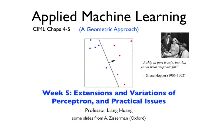
Applied Machine Learning
Professor Liang Huang
Week 5: Extensions and Variations of Perceptron, and Practical Issues
CIML Chaps 4-5
(A Geometric Approach)
“A ship in port is safe, but that is not what ships are for.” – Grace Hopper (1906-1992)
some slides from A. Zisserman (Oxford)