SLIDE 16
- Quantumly, complexity is √N queries
always, all the way up to k=N (i.e., evaluating OR(x1,…,xN), Grover search)
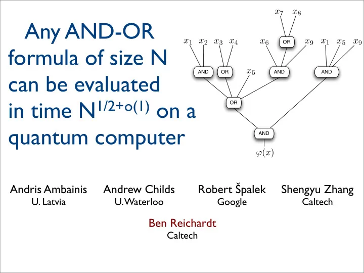
- General AND-OR formulas can be
evaluated with N½+o(1) queries
- Expanding MAJ3 into AND-OR gates
gives O(√5d) quantumly.
- Also, the algorithm generalizes to give
- ptimal algorithm for evaluating
iterated f, where f is any 3-bit function
[Jayram, Kumar, Sivakumar ’03]
- Classical complexity of evaluating
balanced k-ary alternating AND- OR tree is (k/2)depth = N~(1-1/log2k) — approaches N as k increases
evaluating general AND-OR formulas is not known?
- Classical complexity of evaluating
iterative MAJ3 formula is unknown: between and
- (the generalization of the optimal
AND-OR algorithm is not optimal when applied to MAJ3 trees)
Remarks on formula evaluation algorithms: Classical vs. Quantum
Ω
d
d