Analysis of Gene Regulation Networks Using Finite-Field Models - PowerPoint PPT Presentation
Analysis of Gene Regulation Networks Using Finite-Field Models Humberto Ortiz Zuazaga November 29, 2005 1 Background 2 A Model Cell 3 Post Genome Biology or, Ive got all the genes, now what do I do with them? 4 Reverse
Analysis of Gene Regulation Networks Using Finite-Field Models Humberto Ortiz Zuazaga November 29, 2005 1
Background 2
A Model Cell 3
Post Genome Biology or, “I’ve got all the genes, now what do I do with them?” 4
Reverse Engineering Genetic Networks • Input: – A set of genes – A set of gene expression measurements • Output: – A set of control functions by which some genes control others 5
Boolean Genetic Networks 2 4 = 1 f 1 = 1 f 2 = f 3 x 1 ∧ x 2 1 3 f 4 = x 2 ∧ ¬ x 3 6
Boolean Genetic Network Model We define Boolean genetic network model (BGNM): • A Boolean variable takes the values 0, 1. • A Boolean function is a function of Boolean variables, using the operations ∧ , ∨ , ¬ . A Boolean genetic network model (BGNM) is: • An n -tuple of Boolean variables ( x 1 , . . . , x n ) associated with the genes • An n -tuple of Boolean control functions ( f 1 , . . . , f n ), describ- ing how the genes are regulated 7
Reverse Engineering Boolean Networks • Akutsu, S. Kuahara, T. Maruyama, O. Miyano, S. 1998. Identification of gene regulatory networks by strategic gene disruptions and gene overexpressions. Proceedings of the 9th ACM-SIAM Symposium on Discrete Algorithms (SODA 98), H. Karloff, ed. ACM Press. • Ideker, T.E., Thorsson, V., and Karp, R.M. 2000. Discovery of regulatory interactions through perturbation: inference and experimental design. Pacific Symposium on Biocom- puting 5:302-313. • S. Liang, S. Fuhrman and R. Somogyi. 1998. REVEAL, A General Reverse Engineering Algorithm for Inference of Genetic Network Architectures. Pacific Symposium on Bio- computing 3:18-29. 8
Boolean results • Problem: Consistent assignment • Input: a gene network and an assignment of True or False to each variable • Output: True if the assignment is consistent with the rules of the network, False otherwise • Result: Akutsu et al prove this problem is NP-complete (by reduction from 3-SAT) 9
Perturbation experiments • Problem: how many experiments do I need to do? • Input: a gene network with n genes • Output: the number of gene knockdown (force gene to 0) or overexpression (force gene to 1) experiments needed to completely determine the genetic network • Result: worst case, 2 ( n − 1) / 2 • Result: if the degree (number of genes that act on a gene) is limited to D , O ( n 2 D ) Further work proceeds on the assumption that D = 2 or D = 3. 10
Boolean Bugs • Boolean variables can only represent all-or-none effects • Boolean models are deterministic • Efficient algorithms for Boolean networks require indegree of genes to be limited to a small constant value ( i.e., at most 2 or 3 transcription factors act on any given gene) Finite fields represent an alternative algebraic structure to sub- stitute Booleans. Our research seeks to characterize genetic networks based on these fields. 11
Finite field models • Each gene can be an element of a finite field • Multivariate polynomial models • Based on computing Gr¨ oebner bases and ideals Laubenbacher, R. and Stigler, B. (2004), ‘A computational al- gebra approach to the reverse engineering of gene regulatory networks’, J. Theor. Biol. 229 , 523–537. 12
Finite Fields A finite field { F, + , ·} is a finite set F , and two operations + and · that satisfy the following properties: • ∀ a, b ∈ F , a + b ∈ F , a · b ∈ F • ∀ a, b ∈ F , a + b = b + a , a · b = b · a • ∀ a, b, c ∈ F , a + ( b + c ) = ( a + b ) + c , ( a · b ) · c = a · ( b · c ) • ∀ a, b, c ∈ F , a · ( b + c ) = ( a · b ) + ( a · c ) • ∃ 0 , 1 ∈ F , a + 0 = 0 + a = a , a · 1 = 1 · a = a • ∀ a ∈ F , ∃ ( − a ) ∈ F s.t. a + ( − a ) = ( − a ) + a = 0 ∀ a � = 0 ∈ F, ∃ a − 1 ∈ F s.t. a · a − 1 = a − 1 · a = 1 13
The World’s Smallest Finite Field The integers 0 and 1, with integer addition and multiplication modulo 2 form the finite field Z 2 = {{ 0 , 1 } , + , ·} . The operators + and · are defined as follows: + 0 1 · 0 1 0 0 1 0 0 0 1 1 0 1 0 1 14
Products of Sums and Sums of Products We can realize any Boolean function as an expression over Z 2 : X ∧ Y = X · Y X ∨ Y = X + Y + X · Y ¬ X = 1 + X This perspective unites the mathematical foundation of finite fields with the logic of Boolean networks, but remaining within the realm of communications science. 15
Probabilistic Boolean Networks • Each gene may have many controlling functions, select among them by random process. • Generate predictors by enumerating all k -input functions for each gene, tractability requires restricting k to a small inte- ger (4) • Selection probabilities proportional to coefficient of deter- mination of the given gene by a predictor Shmulevich, I., Dougherty, E. R., Kim, S. and Zhang, W. (2002), ‘Probabilistic boolean networks: a rule-based uncertainty model for gene regulatory networks’, Bioinformatics 18 (2), 261–274. 16
Probabilistic Sequential Systems • Generalize BPN to GF( p ) • Combine sequential dynamical systems and PBN Avi˜ n´ o, M. A., Bulancea, G. and Moreno, O. (2005), Probabilis- tic sequential systems, in ‘Proceedings GENSISP’. 17
Conditioned taste aversion (CTA) • associative aversive conditioning paradigm • Animals are exposed to a novel taste, the conditioned stim- ulus • An unconditioned stimulus induces malaise • The animals develop a long lasting aversion to the condi- tioned stimulus 18
CTA Dataset • two controls, the pre-treatment group and the one hour saline group • four time points, 1, 3, 6, and 24 hours after conditioning • 1185 genes on each spotted array • 5 biological replicates of each array Chiesa, R., Ortiz-Zuazaga, H. G., Ge, H. and Pe˜ na de Ortiz, S. (2000), Gene expression profiling in emotional learning with cDNA microarrays, in ‘40th meeting of the American Society for Cell Biology’, San Francisco, California. 19
Objectives and Preliminary Results 20
Objectives 1. To develop new algorithms and heuristics for clustering and error correction, building on finite field models of gene ex- pression networks, and majority logic decoding. 2. To develop new algorithms and heuristics for reverse engi- neering probabilistic models, extending univariate polynomial finite field models 21
Objective 1 To develop new algorithms and heuristics for clustering and error correction, building on finite field models of gene expression networks, and majority logic decoding 22
Finite Field Genetic Networks Any BGNM can be converted into an equivalent model over Z 2 by realizing the boolean functions as sums-of-products and products-of-sums. We now have a finite field genetic network (FFGN): • An n -tuple of variables over Z 2 , ( x 1 , . . . , x n ) associated with the genes • An n -tuple of functions over Z 2 , ( f 1 , . . . , f n ), describing how the genes are regulated Revrese engineering can be done using Lagrange interpolation of univariate polynomials from the time series data. Moreno, O., Ortiz-Zuazaga, H., Corrada Bravo, C. J., Avi˜ n´ o- Diaz, M. A. and Bollman, D. (2004), ‘A finite field deterministic genetic network model’, Preprint. 23
FFGN Models • Finite field models are an improvement on Boolean network models • Laubenbacher’s multivariate polynomial representation of net- works utilizes Gr¨ oebner bases, a somewhat esoteric area • Bollman and Orozco have demonstrated that multivariate and univarite polynomial models are equivalent • Our approach is to bring the tools of modern communica- tions science to bear on the problem of analyzing regularoty networks Bollman, D. and Orozco, E. (2005), Finite field models for genetic networks. Preprint. 24
Error correction A01a glypican 1; HSPG M12; nervous system cell-surface hep- aran sulfate proteoglycan Repetition Pre Sal 1 h 3 h 6 h 24h 1 0.172 0.099 0.176 0.142 0.062 0.152 2 0.274 0.168 0.126 0.114 0.104 0.276 3 0.003 0.119 0.552 0.178 0.193 0.114 4 0.114 0.139 0.6 0.311 0.179 0.181 5 0.04 0.006 0.172 0.103 0.036 -0.047 average 0.121 0.106 0.325 0.17 0.115 0.135 control 0.113 epsilon 0.022 calls + + 0 0 25
Majority logic Repetition 1 h 3 h 6 h 24h 1 + 0 − 0 2 − − − + 3 + + + + 4 + + + + 5 + + 0 − consensus + + ? + 26
Substituting averaged controls Repetition 1 h 3 h 6 h 24h 1 + + − + 2 0 0 0 + 3 + + + 0 4 + + + + 5 + 0 − − cvac + + ? + 27
Pruning extreme values Repetition Pre Sal 1 h 3 h 6 h 24h 1 — 0.099 0.176 0.142 — 0.152 2 — — 0.126 0.114 0.104 — 3 0.003 0.119 — — 0.193 0.114 4 0.114 0.139 — — 0.179 0.181 5 0.04 — 0.172 0.103 — — new average 0.052 0.119 0.158 0.12 0.159 0.149 new control 0.086 new epsilon 0.063 new calls + 0 + 0 28
Consistent calls 1. at least two of the above set of calls agrees in the last 4 columns of data (1 h, 3 h, 6 h, and 24h) 2. either the 1 h or the 24 h columns is a “0” 3. across the last 4 columns of data, the column exhibits the consecutive zeros property ( i.e., values do not oscillate be- tween “0” and “+” or “ − ”) 29
A01a is not consistent 1 h 3 h 6 h 24h average calls + + 0 0 consensus + + ? + cvac + + ? + new calls + 0 + 0 30
Recommend
More recommend
Explore More Topics
Stay informed with curated content and fresh updates.
